Chapter 18 Recursive Mean-Split Estimation

Part V of the book turns from probability representation and inference to nonparametric estimation. The goal of estimation is to recover unknown functional relationships from data without imposing a predetermined parametric form.

A central object in many statistical problems is the conditional mean function

\[ f(x) = E[Y \mid X = x]. \]

Classical regression models estimate this relationship by specifying a functional form — linear, polynomial, or otherwise — and fitting parameters to the data.

Nonparametric methods instead estimate \(f(x)\) directly from observations. Partition-based estimators are among the most intuitive approaches: the predictor space is divided into regions, and the conditional mean is estimated locally within each region.

This chapter introduces the recursive mean-split estimator, the partition-based nonparametric method at the core of the NNS framework. The estimator recursively divides the data into regions based on conditional mean structure, producing a flexible estimator that adapts automatically to nonlinear relationships.

Two distinct splitting modes are available. In joint partitioning, regions are defined by splitting simultaneously on both the predictor \(X\) and the response \(Y\) at their joint means, producing four partial-moment quadrants at each level. In \(X\)-only partitioning, regions are defined by splitting solely on the predictor mean, producing two subregions at each level. Both modes share the same limit condition and recursive logic; they differ in how region boundaries are located and how many subregions each split creates.

The procedure reflects the same directional logic used throughout the book: just as variance decomposes into directional components relative to a benchmark, recursive mean splitting partitions the joint distribution according to deviations around conditional means.

A key theoretical result is established here: the recursive mean-split estimator belongs to the well-studied class of data-adaptive partition estimators, and consistency is inherited directly from that class under standard conditions on cell diameter and occupancy. This is not a limitation requiring further development — it is a strength. The estimator sits within a family whose convergence properties are fully characterized in the literature, and the NNS contribution is the specific splitting rule, the partial-moment geometric interpretation, and the multivariate architecture built on top of that foundation.

---

18.1 Motivation for Partition-Based Estimation

Suppose we observe independent pairs

\[ (X_1, Y_1), \dots, (X_n, Y_n), \]

where

\[ Y_i = f(X_i) + \varepsilon_i, \]

and

\[ E[\varepsilon_i \mid X_i] = 0. \]

The objective is to estimate the unknown regression function

\[ f(x) = E[Y \mid X = x]. \]

18.1.1 Parametric approaches

Parametric regression assumes a functional form such as

\[ f(x) = \beta_0 + \beta_1 x. \]

While simple and interpretable, this assumption can be severely restrictive when the relationship between variables is nonlinear.

18.1.2 Nonparametric alternatives

Nonparametric estimators relax these assumptions. Common examples include

• kernel regression,
• local polynomial regression,
• partition estimators.

Kernel methods estimate \(f(x)\) through weighted averages of nearby observations. However, they require selecting a bandwidth parameter that determines the smoothing scale, and the probability that any kernel function assigns positive mass to an exact observed value is zero — the estimate therefore cannot achieve an exact fit at all observations simultaneously.

Partition estimators divide the predictor space into regions and compute averages within each region. The recursive mean-split method belongs to this class but differs from classical approaches through its partial-moment splitting rule, which anchors region boundaries directly to the geometry of the conditional mean. The estimator is consistent for the true conditional mean under the same regularity conditions that govern all partition estimators in this class — conditions whose sufficiency has been established in the statistical literature. As the order parameter increases, the number of regions grows and the estimator converges to a perfect fit in finite steps.

---

18.2 Consistency by Class Membership

The recursive mean-split estimator is an instance of the data-adaptive partition estimator class studied by Stone (1977), Lugosi and Nobel (1996), and Györfi, Kohler, Krzyżak, and Walk (2002).

The general result for this class is as follows.

Theorem (Consistency of Partition Estimators). Let \((X_1, Y_1), \dots, (X_n, Y_n)\) be independent and identically distributed, with \(E[Y^2] < \infty\). Let \(\hat{f}_n\) be the partition estimator

\[ \hat{f}_n(x) = \frac{1}{N_{n,x}} \sum_{i : X_i \in A_n(x)} Y_i, \]

where \(A_n(x)\) is the cell of a data-adaptive partition \(\mathcal{P}_n\) containing \(x\). If the partition satisfies

\[ \operatorname{diam}(A_n(x)) \xrightarrow{P} 0 \qquad \text{and} \qquad N_{n,x} \xrightarrow{P} \infty \]

as \(n \to \infty\), then

\[ E\bigl[(\hat{f}_n(x) - f(x))^2\bigr] \to 0. \]

The recursive mean-split estimator satisfies both conditions under the standard occupancy and order growth assumptions used in practice. As \(n \to \infty\) with order parameter \(O = O(n)\) growing appropriately and minimum occupancy held fixed:

• each cell’s diameter converges to zero because successive splits are anchored to sample means, which concentrate around the true conditional mean as \(n\) grows, producing finer and finer partitions in regions where the function varies;
• each cell’s occupancy grows because the data density in any fixed region of the predictor space grows linearly with \(n\).

Consequently, consistency of the recursive mean-split estimator is inherited directly from the established theory of partition estimators. This is not an approximate or informal claim. The estimator belongs to a well-characterized class, and the convergence result applies.

What the NNS framework contributes beyond this class membership is:

1. a specific splitting rule grounded in the partial-moment geometry of the data,
2. a finite-order perfect-fit property unavailable to kernel estimators,
3. a multivariate architecture — developed fully in Chapter 21 — that operates on per-regressor regression points rather than on the raw observation cloud, substantially mitigating the curse of dimensionality.

---

18.3 Conditional Mean Partitions

Let \(P_n\) denote a partition of the data space into regions

\[ A_1, A_2, \dots, A_K. \]

Within each region, the conditional mean is estimated by averaging the responses of observations whose predictors fall inside that region.

For a predictor value \(x\), let

\[ A_n(x) \]

be the cell containing \(x\). The partition estimator is

\[ \hat{f}_n(x) = \frac{1}{N_{n,x}} \sum_{i : X_i \in A_n(x)} Y_i, \]

where

\[ N_{n,x} = \#\{ i : X_i \in A_n(x) \} \]

is the number of observations in the cell.

The estimate of \(f(x)\) is therefore the average response within the region containing \(x\).

This structure is flexible in three respects:

• Regions adapt to nonlinear features of the conditional mean surface.
• Local averages approximate the conditional expectation without a specified functional form.
• Estimation is entirely data-driven.

The size and shape of regions determine the effective smoothing scale: coarser regions produce smoother estimates; finer regions track local variation more closely.

---

18.4 Recursive Splitting Algorithms

The key design choice is how the regions \(A_k\) are constructed.

The NNS recursive mean-split estimator builds partitions through an iterative procedure governed by an order parameter \(O\). At each order, each existing region is further subdivided. When left unspecified in the package interface (order = NULL), recursion depth is determined internally for each regressor according to its directional dependence with the response; Chapter 21 formalizes this dependence-driven adaptivity in the regression workflow.

Two splitting modes are available, depending on whether regions are anchored to the joint distribution of \((X, Y)\) or to the marginal distribution of \(X\) alone.

---

18.5 Joint Partitioning

Joint partitioning defines regions by splitting simultaneously on both \(X\) and \(Y\) at their local means.

18.5.1 Initialization

Begin with all \(n\) observations as a single region.

18.5.2 Splitting rule

For a region \(R\) containing observations \(\{(X_i, Y_i)\}_{i \in I_R}\), compute the local means

\[ \bar{X}_R = \frac{1}{|I_R|} \sum_{i \in I_R} X_i, \qquad \bar{Y}_R = \frac{1}{|I_R|} \sum_{i \in I_R} Y_i. \]

Partition the observations in \(R\) into four quadrants according to whether each observation lies above or below \(\bar{X}_R\) and \(\bar{Y}_R\):

Quadrant	Condition	Label
CoUPM	\(X_i > \bar{X}_R\) and \(Y_i > \bar{Y}_R\)	NE
DUPM	\(X_i \le \bar{X}_R\) and \(Y_i > \bar{Y}_R\)	NW
DLPM	\(X_i > \bar{X}_R\) and \(Y_i \le \bar{Y}_R\)	SE
CoLPM	\(X_i \le \bar{X}_R\) and \(Y_i \le \bar{Y}_R\)	SW

These four quadrants correspond directly to the four co-partial moment regions introduced in Chapter 10. The joint mean \((\bar{X}_R, \bar{Y}_R)\) is the point at which

\[ U_1(\bar{X}_R; X \mid R) = L_1(\bar{X}_R; X \mid R) \quad \text{and} \quad U_1(\bar{Y}_R; Y \mid R) = L_1(\bar{Y}_R; Y \mid R), \]

so the split occurs precisely where the first-order upper and lower partial moments are balanced on both dimensions. Each observation is assigned to one of the four quadrants, with a quadrant identification number recorded at each level.

18.5.3 Recursion

Within each nonempty quadrant, repeat the same procedure: compute local means and split into four subquadrants. Continuing to order \(O\) produces at most \(4^{O-1}\) nonempty regions.

18.5.4 Regression points

The regression points of the partition are the local means \((\bar{X}_R, \bar{Y}_R)\) within each region. These points summarize the conditional mean surface and serve as the basis for prediction and curve fitting.

x <- seq(-5, 5, .05)
y <- x ^ 3

for(i in 1 : 4){NNS.part(x, y, order = i, Voronoi = TRUE, obs.req = 0)}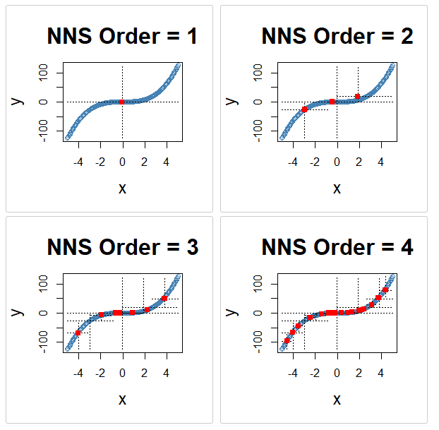

Figure 18.1. NNS.part joint partitioning for orders 1–4 (Voronoi view), showing progressive recursive refinement.

---

18.6 \(X\)-Only Partitioning

\(X\)-only partitioning defines regions by splitting solely on the mean of the predictor \(X\), without reference to \(Y\).

18.6.1 Initialization

Begin with all \(n\) observations as a single region.

18.6.2 Splitting rule

For a region \(R\) with observations \(\{(X_i, Y_i)\}_{i \in I_R}\), compute the local predictor mean

\[ \bar{X}_R = \frac{1}{|I_R|} \sum_{i \in I_R} X_i. \]

Partition the observations into two subregions:

\[ R_L = \{ i \in I_R : X_i \le \bar{X}_R \}, \qquad R_U = \{ i \in I_R : X_i > \bar{X}_R \}. \]

Quadrant identifications in this mode are limited to the symbols 1 (left of the split) and 2 (right of the split).

18.6.3 Recursion

Within each nonempty subregion, repeat the same procedure. Continuing to order \(O\) produces at most \(2^O\) nonempty regions.

18.6.4 Regression points

The regression points are the local means \((\bar{X}_R, \bar{Y}_R)\) within each predictor-defined region. Because the region boundaries are determined by \(X\) alone, the regression points make use of the full bandwidth of the response values within each region for their \(Y\) coordinate.

x <- seq(-5, 5, .05)
y <- x ^ 3

for(i in 1 : 4){NNS.part(x, y, order = i, type = "XONLY", Voronoi = TRUE, obs.req = 0)}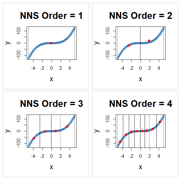

Figure 18.2. NNS.part(..., type = "XONLY") predictor-only partitioning across recursive splits.

---

18.7 Comparison of Modes

Both modes share the same conceptual foundation — recursive splitting at local means — and converge to a perfect fit as \(O\) grows. They differ in the following respects.

Property	Joint partitioning	\(X\)-only partitioning
Split dimensions	\(X\) and \(Y\) jointly	\(X\) only
Subregions per split	4	2
Regions at order \(O\)	at most \(4^{O-1}\)	at most \(2^O\)
Quadrant IDs	digits 1–4	digits 1–2
Region definition	Joint (X,Y) partial-moment quadrants	Predictor-space intervals
Regression points	Joint quadrant means	Predictor-interval means

Joint partitioning converges faster due to exponential growth in regions and provides a richer representation of the joint distribution. \(X\)-only partitioning is more directly analogous to classical predictor-space partition estimators and is often preferred when a clear functional relationship \(Y = f(X)\) is the primary object of interest.

18.7.1 Stopping criteria

Splitting terminates when any of the following conditions are met:

• A region contains fewer than a user-specified minimum number of observations (minimum occupancy threshold).
• The order parameter \(O\) reaches a user-specified maximum.

The minimum occupancy threshold is quantitative and directly governs the coarsest admissible partition. Under any fixed occupancy threshold, as \(n \to \infty\) the occupied regions shrink and the occupancy within each region grows, satisfying the two conditions required for consistency in the partition estimator class.

---

18.8 Partial-Moment Interpretation of Joint Partitioning

The joint splitting rule has a precise interpretation in terms of the partial-moment framework developed in earlier chapters.

Recall from Chapter 5 that variance decomposes into directional components:

\[ \text{Var}(X) = U_2(\mu_X; X) + L_2(\mu_X; X), \]

where

\[ U_2(\mu_X; X) = E[(X - \mu_X)_+^2] \quad \text{and} \quad L_2(\mu_X; X) = E[(\mu_X - X)_+^2]. \]

Recursive joint splitting applies this logic at the level of the conditional distribution within each region.

Each split separates observations into four directional groups defined by their co-partial-moment quadrant membership — the same four regions introduced in Chapter 10:

• CoUPM: above \(\bar{X}_R\) and above \(\bar{Y}_R\),
• CoLPM: below \(\bar{X}_R\) and below \(\bar{Y}_R\),
• DLPM: above \(\bar{X}_R\) and below \(\bar{Y}_R\),
• DUPM: below \(\bar{X}_R\) and above \(\bar{Y}_R\).

The joint mean \((\bar{X}_R, \bar{Y}_R)\) is the unique point at which the first-order partial moments balance on both axes. Splitting at this point therefore exactly decomposes the local joint variability into its four directional components.

By recursively applying this decomposition, the algorithm parses the joint distribution into regions of progressively refined directional structure. Areas where the conditional mean changes most rapidly — where the CoUPM and CoLPM quadrants are most unequal in their response means — are split more frequently as \(O\) increases, because the local means shift and the quadrant boundaries realign at each level.

The resulting partition structure therefore reflects the geometry of the conditional mean surface, not an externally imposed grid.

---

18.9 Multivariate Predictors

For a predictor vector \(X_i \in \mathbb{R}^d\), the recursive mean-split procedure extends through an architecture designed specifically to mitigate the curse of dimensionality. This architecture is described in full in Chapter 21; its foundations are laid here.

18.9.1 Per-regressor partitioning against the response

The key structural decision in the multivariate case is that each predictor is partitioned independently against the response, rather than partitioning the joint predictor space.

For predictor \(j \in \{1, \dots, d\}\ \), recursive mean splitting is applied to the pairs \((X_i^{(j)}, Y_i)\) to produce a set of regression points for that predictor — local conditional means summarizing the relationship between \(X^{(j)}\) and \(Y\). These per-regressor partitions are each governed by the same splitting rules described above and produce a set of \(K_j\) regression points for predictor \(j\).

This is not joint partitioning of the full \(d\)-dimensional predictor space. It is a collection of univariate partitions, each anchored to the response. The important consequence is that the number of candidate regression points grows as \(\sum_j K_j\) — linearly in the number of regressors — rather than as \(\prod_j K_j\), which would grow exponentially and reproduce the curse.

18.9.2 Regression point matrix

The regression points from all \(d\) per-regressor partitions are assembled into a regression point matrix (RPM). Each row of the RPM corresponds to one occupied joint region in the multivariate structure; the columns record the local mean of each predictor within that region, and a final column records the corresponding local mean response.

For a new observation \(x^* \in \mathbb{R}^d\), prediction proceeds by identifying the rows of the RPM closest to \(x^*\) across the predictor columns, then returning the distance-weighted average of the corresponding local response means. This is a nearest-neighbor search over regression points — compressed, denoised local conditional means — rather than over the \(n\) raw observations.

The curse of dimensionality is mitigated along two dimensions simultaneously:

1. Search space compression. The RPM has far fewer rows than \(n\). Each row is a local conditional mean derived from a cluster of observations, not a raw data point.
2. Noise reduction before search. Each regression point has already been smoothed through local averaging, so the candidates in the nearest-neighbor search carry substantially less noise than raw observations.

The full multivariate prediction architecture — including dependence-adaptive neighbor count and alternative synthetic-predictor dimension reduction — is developed in Chapter 21.

---

18.10 Estimation Workflow

In practice, recursive mean-split estimation follows a direct workflow.

18.10.1 Step 1 — Data preparation

Collect paired observations

\[ (X_i, Y_i), \quad i = 1, \dots, n, \]

with \(X_i \in \mathbb{R}^d\) for the multivariate case.

18.10.2 Step 2 — Select partitioning mode

Choose joint partitioning (using both \(X\) and \(Y\) means) or \(X\)-only partitioning (using only the predictor mean), depending on the application.

18.10.3 Step 3 — Recursive mean splitting

Iteratively apply the mean-split rule:

1. Compute the local conditional means within the region.
2. Divide observations according to their quadrant membership.
3. Assign quadrant identifications and record regression points.
4. Repeat within each subregion.

18.10.4 Step 4 — Stopping rule

Terminate splitting when any region falls below the minimum occupancy threshold or when the order \(O\) reaches its maximum.

18.10.5 Step 5 — Prediction

For a new predictor value \(x\):

1. Identify the region \(A_n(x)\) containing \(x\) (univariate) or the matching rows in the RPM (multivariate).
2. Return the local response mean or the distance-weighted average of the nearest regression-point means as the predicted value:

\[ \hat{f}_n(x) = \frac{1}{N_{n,x}} \sum_{i : X_i \in A_n(x)} Y_i. \]

18.10.6 Step 6 — Curve fitting (optional)

The regression points at each order can be connected by linear segments to produce a piecewise-linear curve. This provides a smooth interpolating surface between partition means, supports well-defined interpolation and extrapolation, and reduces variance relative to a pure step-function estimator.

---

18.11 Limit Condition and Perfect Fit

A notable property of the recursive mean-split estimator is its finite-order limit condition.

As the order \(O\) increases, the number of regions grows — exponentially in the joint case (\(4^{O-1}\)) or geometrically in the \(X\)-only case (\(2^O\)). At a finite order \(O^*\), every observation occupies its own region and becomes its own regression point. At this limit:

\[ \hat{f}_n(X_i) = Y_i \quad \text{for all } i = 1, \dots, n, \]

and the \(R^2\) of the in-sample fit equals 1.

This property distinguishes NNS from kernel regression, which cannot achieve an exact fit at all observations simultaneously due to the continuous support of the kernel function. The limit condition is reached in finite steps, not asymptotically.

In practice, \(O\) is selected to balance fit quality against overfitting. Larger \(O\) reduces bias but increases variance; the appropriate order is determined by the signal-to-noise ratio of the data. The NNS dependence measure provides an objective criterion for this selection.

---

18.12 Properties of the Recursive Mean-Split Estimator

The recursive mean-split estimator possesses several important characteristics.

18.12.1 Consistency by class inheritance

The estimator belongs to the class of data-adaptive partition estimators studied by Stone (1977) and extended by Lugosi and Nobel (1996) and Györfi et al. (2002). Under standard conditions — shrinking cell diameter and growing cell occupancy — the class is universally consistent. The recursive mean-split estimator satisfies these conditions under the occupancy and order growth rules used in practice, and consistency is therefore established by class membership rather than requiring a separate proof from first principles.

18.12.2 Nonparametric flexibility

No functional form is imposed on the relationship between \(X\) and \(Y\). The estimator represents highly nonlinear relationships without specifying a parametric family.

18.12.3 Grounding in partial moments

Region boundaries are defined by the same partial-moment structure — upper and lower deviations relative to a benchmark — that underlies the directional statistics developed throughout this book. The estimator is therefore not simply an ad hoc tree method but an application of the NNS partial-moment framework to the estimation of conditional expectations.

18.12.4 Data-adaptive partitions

Regions are determined entirely by the data. Areas where the conditional mean changes rapidly receive finer partitions as \(O\) increases.

18.12.5 Implicit smoothing

The order \(O\) governs the effective smoothing scale. Chapter 19 formalizes this by interpreting the partition cell diameter as a dynamic bandwidth, connecting the estimator to classical nonparametric smoothing theory.

18.12.6 Piecewise-linear interpolation

Connecting regression points with line segments produces an interpolating surface that is stable, interpretable, and well-behaved for interpolation and extrapolation — properties that kernel-based nonparametric regressions do not generally share.

18.12.7 Finite limit condition

At a finite order \(O^*\), every observation occupies its own region and the estimator achieves a perfect in-sample fit — \(\hat{f}_n(X_i) = Y_i\) for all \(i\). This property is not available to kernel or polynomial methods, which are intrinsically approximate. It provides a well-defined upper bound on approximation error and a principled spectrum of fits indexed by \(O\), from a single linear approximation at \(O = 1\) to exact interpolation at \(O = O^*\).

---

18.13 Relationship to Other Methods

The recursive mean-split estimator is related to several classical approaches but differs from each in important respects.

18.13.1 CART and decision trees

CART algorithms select splits greedily to minimize impurity or squared prediction error, then apply pruning penalties to prevent overfitting.

Recursive mean splitting differs in two key respects. First, the splitting criterion is the conditional mean of the data within the region, not an optimized impurity measure. Second, overfitting is controlled through the minimum occupancy threshold and the order parameter rather than through post-hoc pruning. The resulting partition structure follows the conditional mean geometry rather than an impurity landscape (Breiman et al., 1984).

18.13.2 Kernel regression

Kernel estimators smooth data using a bandwidth parameter selected externally, often by cross-validation.

Recursive mean-split estimation avoids explicit bandwidth selection: smoothing arises implicitly through the order parameter and the partition cell size. Chapter 19 makes this connection precise by showing that the cell diameter functions as a data-adaptive bandwidth.

A further distinction concerns exactness of fit. Because all kernel functions are continuous probability distributions, the probability that a kernel function assigns positive mass to any exact observed value is zero. Consequently, the kernel estimate at any point is a weighted average over the surrounding distribution and can never exactly equal any single observation. The recursive mean-split estimator does not share this limitation: at finite order \(O^*\), it achieves an exact fit at every observed point simultaneously.

18.13.3 \(k\)-means clustering

The NNS partition objective — minimizing within-quadrant sum of squares — is equivalent to the \(k\)-means objective when the number of clusters equals the number of partition regions. The key difference is that NNS does not require a pre-specified \(k\): the number of regions is determined by the order parameter \(O\) and the data, not by an externally supplied cluster count.

18.13.4 Fixed-grid estimators

Uniform grids divide the predictor space into equally sized cells. Mean-split partitions are data-driven and adapt to the density and conditional mean geometry of the sample.

---

18.14 Summary

Recursive mean-split estimation provides a flexible, data-adaptive, nonparametric method for estimating conditional expectations.

The key ideas developed in this chapter are:

• Consistency by class membership. The recursive mean-split estimator belongs to the class of data-adaptive partition estimators, for which universal consistency under shrinking-diameter and growing-occupancy conditions has been established in the literature (Stone 1977; Lugosi and Nobel 1996; Györfi et al. 2002). The estimator satisfies both conditions under standard stopping rules, and its consistency is therefore inherited directly from this class.
• Partition-based estimation of conditional means, using the local sample average within each region as the estimator.
• Two splitting modes: joint \((X, Y)\) partitioning, which creates four partial-moment quadrants at each split, and \(X\)-only partitioning, which creates two predictor-interval subregions.
• The joint splitting rule is grounded in the co-partial-moment structure of the NNS framework: region boundaries coincide with the joint conditional means, and the four quadrants correspond exactly to the CoUPM, CoLPM, DLPM, and DUPM regions.
• An order parameter \(O\) governs partition depth; at a finite \(O^*\), the estimator achieves a perfect in-sample fit.
• Multivariate predictors are handled via per-regressor partitioning against the response, which produces a regression point matrix (RPM) of local conditional means. The search space for prediction grows linearly in the number of regressors, not exponentially, substantially mitigating the curse of dimensionality.
• Prediction connects regression points with local averages or piecewise-linear segments in the univariate case, and with distance-weighted nearest-neighbor averaging over the RPM in the multivariate case.

Chapter 19 interprets the partition cell diameter as a dynamic bandwidth, linking the estimator to classical kernel smoothing theory while preserving its data-adaptive character.

Chapter 21 develops the multivariate regression architecture in full, showing how per-regressor partitioning with response-anchored centroids — combined with dependence-adaptive neighbor count — produces a nearest-neighbor prediction method over a compressed, denoised geometry that handles high-dimensional predictors substantially better than raw-observation kNN.

---

18.15 References

• Stone, C. J. (1977). Consistent nonparametric regression. Annals of Statistics, 5(4), 595–620.

• Lugosi, G., & Nobel, A. (1996). Consistency of data-driven histogram methods for density estimation and classification. Annals of Statistics, 24(2), 687–706.

• Györfi, L., Kohler, M., Krzyżak, A., & Walk, H. (2002). A Distribution-Free Theory of Nonparametric Regression. Springer.

• Breiman, L., Friedman, J. H., Olshen, R. A., & Stone, C. J. (1984). Classification and Regression Trees. Wadsworth.

• Vinod, H. D., & Viole, F. (2018). Clustering and curve fitting by line segments. Preprints, 2018010090. https://doi.org/10.20944/preprints201801.0090.v1

• Viole, F., & Nawrocki, D. (2012). Deriving nonlinear correlation coefficients from partial moments. SSRN eLibrary. https://doi.org/10.2139/ssrn.2148522

• Viole, F. (2016). NNS: Nonlinear nonparametric statistics. R package. https://cran.r-project.org/package=NNS