Chapter 21 Clustering
Chapters 19–20 developed the recursive mean-split estimator as a partition-based method for nonparametric estimation and showed that its induced cell geometry behaves like a dynamic bandwidth. Those results focused on supervised estimation, where a response variable \(Y\) is observed and the objective is to recover a conditional mean function.
This chapter turns to unsupervised learning.
In unsupervised learning there is no designated response variable. The goal is instead to discover structure within the data itself. Among the most fundamental unsupervised tasks is clustering: partitioning observations into groups whose members are more similar to one another than to members of other groups.
Classical clustering methods such as k-means and hierarchical clustering are widely used, but they inherit familiar limitations:
- k-means is driven by Euclidean distance and spherical-centroid geometry,
- hierarchical clustering depends heavily on linkage rules,
- both require the analyst to specify or assume a number of groups in advance,
- and both can obscure nonlinear, asymmetric, and benchmark-relative structure.
The directional framework developed throughout this book suggests a different perspective.
Rather than defining similarity purely by geometric distance, we can define it through directional behavior relative to local benchmarks. In this view, clustering is not merely grouping by proximity. It is grouping by shared directional structure.
Critically, the number of clusters that emerges from this procedure is determined by the data, not prescribed by the analyst. This is not a minor implementation detail. It is a fundamental departure from methods that require \(K\) to be chosen before any structure has been examined — and it means, in particular, that the number of clusters need not equal, and in general will not equal, the number of class labels in any downstream supervised problem.
This chapter develops that idea using the partition machinery introduced in Chapters 19–20 and connects it to the NNS clustering procedure.
21.1 What Clustering Seeks to Recover
Suppose we observe multivariate data
\[X_1, X_2, \dots, X_n \in \mathbb{R}^d.\]
A clustering algorithm seeks a partition of the index set
\[\{1,2,\dots,n\} = C_1 \cup C_2 \cup \cdots \cup C_K, \qquad C_j \cap C_\ell = \varnothing \text{ for } j \ne \ell,\]
where each set \(C_k\) is interpreted as a cluster.
The ideal is that observations within the same cluster share a common structural pattern, while observations in different clusters do not.
But this raises two immediate questions:
What does “similar” mean?
And equally: how many groups should there be?
Different clustering methods answer both questions differently. Classical methods typically answer the second question first — by requiring the analyst to supply \(K\) — and then optimize toward that prespecified count. The directional framework answers neither question in advance. Similarity is defined through benchmark-relative structure, and the number of clusters is whatever the recursive partition produces under the chosen stopping rule. Crucially, that count is a consequence of the data, not an assumption about it.
- Euclidean methods define similarity through geometric closeness.
- Density methods define similarity through connected regions of high probability mass.
- Model-based methods define similarity through shared latent distributions.
- Directional methods define similarity through shared benchmark-relative structure.
The directional definition is particularly natural when the variables exhibit asymmetry, nonlinear dependence, or tail-specific behavior.
21.2 Why Distance Alone Can Mislead
The simplest clustering intuition is geometric distance.
If two observations \(x_i\) and \(x_j\) are close in Euclidean norm,
\[\|x_i - x_j\|,\]
they are regarded as similar.
This works well when clusters are compact, approximately spherical, and separated mainly by location.
But many real datasets violate these conditions.
21.2.1 Nonlinear shape
Two observations can lie on the same curved manifold and be structurally similar even if their straight-line distance is not especially small.
21.2.2 Asymmetric spread
Clusters may have very different directional variability: wide in one direction, narrow in another.
21.2.3 Benchmark-relative structure
Two points may be similar because they lie on the same side of a threshold across several variables, even if their raw coordinates differ.
21.2.4 Tail co-movement
Observations may be grouped naturally by whether they occur jointly in extreme regions rather than by ordinary central distance.
Distance alone therefore treats all directions symmetrically and all dimensions uniformly unless ad hoc reweighting is imposed.
The directional framework instead asks whether observations share common sign and magnitude of deviation relative to meaningful benchmarks.
21.3 Partition-Based Clustering
The recursive mean-split machinery from Chapter 18 provides a natural unsupervised clustering mechanism.
In supervised estimation, partition cells were used to approximate a regression surface. In clustering, the same recursive partitions can be interpreted directly as unsupervised groupings of the data cloud.
Let \(R\subset \mathbb{R}^d\) denote a region containing a subset of observations. Define the local centroid
\[\bar X_R = \frac{1}{|I_R|}\sum_{i\in I_R} X_i,\]
where \(I_R\) indexes the observations in region \(R\).
The directional idea is to partition the region relative to this local benchmark.
In two dimensions this creates four quadrants. In \(d\) dimensions it creates up to \(2^d\) directional subregions, depending on which coordinates lie above or below their local means.
At each stage:
- compute the local benchmark vector,
- assign each observation according to its directional deviation pattern,
- recurse within each nonempty subregion.
This yields a tree of increasingly refined directional cells.
The terminal cells form a clustering of the data. Their number is determined entirely by where observations fall relative to successive local means and by the chosen stopping rule. No value of \(K\) is ever specified.
Unlike k-means, these clusters are not required to be spherical, convex, or globally separable by Voronoi boundaries. They arise from repeated local directional refinement.
21.4 Clusters Are Not Classes
A point that deserves explicit statement: the number of clusters produced by the directional partition need not equal, and in general will not equal, the number of classes in a downstream classification problem.
This distinction matters because the two concepts serve different purposes.
A cluster is a group of observations that share common benchmark-relative directional structure in the predictor space. It is an unsupervised concept, derived entirely from the geometry of the data cloud without reference to any response variable or label.
A class is a label assigned to an observation — by a supervisor, domain expert, or measured outcome. In a classification problem, classes are given; the analyst’s task is to predict them.
The relationship between clusters and classes is empirical, not definitional. A dataset with 3 known class labels may contain 4, 7, or 12 natural directional clusters, because the feature space harbors more local structure than the labels alone reflect. Conversely, a dataset with 10 nominal categories may collapse to 3 meaningfully distinct directional clusters if several categories share the same benchmark-relative geometry.
Neither outcome is a failure. They reflect the fact that clusters describe where the data lives while classes describe what the data is labeled. The two can inform each other — clusters often predict classes well precisely because shared directional structure tends to co-occur with shared labels — but they are answering different questions.
This matters practically. When using directional partitioning as a preprocessing step for classification, the analyst should not constrain the number of clusters to match the number of known classes. Doing so would import a supervised assumption into an unsupervised procedure and foreclose the possibility of discovering that the data contains more, fewer, or differently arranged groups than the labels suggest. Instead, let the recursive partition discover the natural directional groupings, then examine how class labels distribute across those groups. If clusters map cleanly to classes, that alignment is a finding. If they do not, that misalignment is also informative.
21.5 Directional Similarity
To formalize the idea, let \(x_i, x_j \in \mathbb{R}^d\) be two observations and let \(t \in \mathbb{R}^d\) denote a benchmark vector.
For each coordinate \(m = 1,\dots,d\), define the directional signs
\[s_m(x_i;t) = \begin{cases} -1 & x_{im} \le t_m,\\ +1 & x_{im} > t_m. \end{cases}\]
The vector
\[s(x_i;t) = \bigl(s_1(x_i;t),\dots,s_d(x_i;t)\bigr)\]
records the directional region occupied by \(x_i\) relative to the benchmark.
Two observations are directionally concordant at benchmark \(t\) if
\[s(x_i;t) = s(x_j;t).\]
They are directionally discordant if they occupy different sign regions.
This already gives a coarse notion of similarity: observations falling into the same directional cell share the same pattern of benchmark-relative deviations.
A richer notion includes magnitudes. Define the directional deviation vectors
\[u(x_i;t) = \bigl((x_{i1}-t_1)_+,\dots,(x_{id}-t_d)_+\bigr),\]
\[\ell(x_i;t) = \bigl((t_1-x_{i1})_+,\dots,(t_d-x_{id})_+\bigr).\]
These separate upward and downward deviations coordinatewise. Two observations can then be judged similar not only because they lie in the same directional region, but because their directional deviation magnitudes are similar.
This is the unsupervised analogue of the partial-moment logic used throughout the book.
21.6 Recursive Mean Splits as Unsupervised Structure Discovery
The recursive clustering logic can be understood most clearly in low dimension.
21.6.1 Two-dimensional case
Suppose each observation is a pair
\[X_i = (X_{i1}, X_{i2}).\]
Within a region \(R\), compute the local mean vector
\[(\bar X_{R,1}, \bar X_{R,2}).\]
This mean induces four directional regions:
| Region | Condition |
|---|---|
| lower-lower | \(X_{i1}\le \bar X_{R,1}\), \(X_{i2}\le \bar X_{R,2}\) |
| lower-upper | \(X_{i1}\le \bar X_{R,1}\), \(X_{i2}> \bar X_{R,2}\) |
| upper-lower | \(X_{i1}> \bar X_{R,1}\), \(X_{i2}\le \bar X_{R,2}\) |
| upper-upper | \(X_{i1}> \bar X_{R,1}\), \(X_{i2}> \bar X_{R,2}\) |
Each nonempty region is then split again using its own local mean.
This process produces a nested partition of the data cloud.
21.6.2 Higher-dimensional case
In \(d\) dimensions the same principle applies, though the number of directional subregions per split can grow to \(2^d\). In practice one often works with lower-dimensional projections, selected variable subsets, or stopping rules that prevent excessive fragmentation.
The core idea remains unchanged:
cluster structure is revealed by repeated directional partitioning around local benchmarks.
This is unsupervised because no response variable is needed. The geometry of the predictor cloud is itself the object of analysis. And the number of clusters that results is a property of that geometry — not a parameter set in advance.
21.7 Relationship to Partial Moments
The connection to partial moments is more than intuitive.
Recall from earlier chapters that benchmark-relative structure is encoded by directional deviation operators. In clustering, those same operators summarize the local spread of each candidate cluster.
For a region \(R\) and coordinate \(m\), define local partial moments about the regional mean \(t_m = \bar X_{R,m}\):
\[U_r^{(R,m)} = \frac{1}{|I_R|}\sum_{i\in I_R}(X_{im}-\bar X_{R,m})_+^r,\]
\[L_r^{(R,m)} = \frac{1}{|I_R|}\sum_{i\in I_R}(\bar X_{R,m}-X_{im})_+^r.\]
These quantities describe the directional spread of the cluster in each coordinate.
A region with balanced and small directional moments is relatively compact around its centroid. A region with large or highly asymmetric directional moments is more diffuse and may warrant further splitting.
Thus recursive clustering can be interpreted as repeatedly refining regions whose directional spread remains structurally heterogeneous.
In this way, clustering is tied directly to the same benchmark-relative decomposition that generated classical moments and dependence measures earlier in the book.
21.8 Comparison with k-Means
The most common partition-based clustering method is k-means.
Given a desired number of clusters \(K\), k-means minimizes the within-cluster sum of squared Euclidean distances:
\[\sum_{k=1}^K \sum_{i\in C_k} \|x_i - \mu_k\|^2,\]
where \(\mu_k\) is the centroid of cluster \(C_k\).
This objective has several advantages:
- computational simplicity,
- interpretability,
- good performance for compact spherical clusters.
But it also has well-known limitations.
21.8.1 Prespecified \(K\)
The number of clusters must be chosen in advance. This is the most fundamental limitation: the analyst must decide how many groups exist before examining whether the data supports that count.
21.8.2 Euclidean symmetry
The method is driven by squared symmetric distance and therefore inherits the same aggregation logic criticized in earlier chapters.
21.8.4 Sensitivity to initialization
Different random starts can produce different solutions.
The directional partition approach differs in all four respects.
- It generates a hierarchy of clusters without requiring a fixed \(K\) at the outset. The number of terminal clusters is a derived quantity, not an input.
- It partitions by directional benchmark-relative structure rather than global squared distance alone.
- It accommodates irregular, asymmetric, and locally nonlinear cluster geometry.
- Its recursion is deterministic once the splitting rule and stopping criteria are specified.
The contrast on the first point is worth dwelling on. When an analyst runs k-means with \(K = 3\) because a dataset has 3 known classes, they have already imported supervised information into an unsupervised procedure. The directional framework keeps the two tasks separate: discover how many directional groups the data contains, then examine how those groups relate to any available labels. These are different questions, and conflating them by setting \(K\) equal to the number of classes forecloses the possibility of learning anything surprising from the unsupervised step.
This does not imply that directional clustering dominates k-means in every setting. If the true cluster structure is spherical and centroid-based, k-means is efficient and appropriate. The point is that many real datasets are not, and that a data-determined \(K\) is almost always preferable to an analyst-assumed one.
# Clustered Dataset
g <- 6
set.seed(g)
n <- 100
d <- data.frame(x = unlist(lapply(1:g, function(i) rnorm(n/g, runif(1)*i^2))),
y <- unlist(lapply(1:g, function(i) rnorm(n/g, runif(1)*i^2))))

library(clue)
par(mfrow = c(2, 1))
km <- kmeans(d, 3)
plot(d, col = km$cluster, main = paste("k-means (k = ", 3,")", sep = ""),
     cex.main = 2)
points(km$centers, pch = 15, col = 3:1)
NNS.part(d$x, d$y, order = 3, Voronoi = TRUE, obs.req = 0)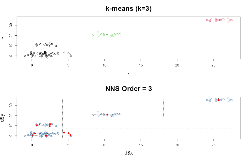
21.9 Comparison with Hierarchical Clustering
Hierarchical clustering constructs nested groupings either by
- agglomeration: successively merging points or clusters, or
- division: successively splitting them.
Its main attraction is that it yields a dendrogram rather than a single partition, and it does not require \(K\) to be fixed before the algorithm runs — the analyst cuts the tree at a chosen height after the fact.
However, hierarchical clustering depends heavily on the chosen linkage rule:
- single linkage,
- complete linkage,
- average linkage,
- Ward’s method.
Different linkage rules can produce very different cluster structures on the same data.
The directional recursive partition procedure is also hierarchical and also avoids fixing \(K\) in advance. But its hierarchy is built from local benchmark splits rather than pairwise merge criteria.
This yields several conceptual differences.
21.9.1 Geometry
Hierarchical distance methods are governed by pairwise distances. Directional recursion is governed by local benchmark-relative partitions.
21.9.2 Interpretation
Dendrogram merges may be difficult to interpret substantively. Directional splits are interpretable as above-below benchmark separations along specific coordinates or regions.
21.9.3 Local adaptivity
Directional recursion recomputes local means inside each region, allowing the geometry to adapt as the partition deepens.
Thus directional clustering can be viewed as a benchmark-driven divisive hierarchical method whose effective \(K\) is determined by stopping criteria applied to local directional spread rather than by visual inspection of a dendrogram.
21.10 Stopping Rules and Practical Cluster Formation
A recursive partition procedure requires a stopping rule. Otherwise it eventually isolates individual observations into singleton clusters — the maximum possible \(K\), and the least useful.
Several stopping criteria are natural. Each implicitly determines how many clusters the procedure returns.
21.10.1 Minimum cell size
Stop splitting when a region contains fewer than some threshold number of observations. This directly bounds the finest possible partition and places a floor on cluster size.
21.10.2 Maximum order
Stop after a fixed recursion depth. At order \(O\), the maximum number of populated terminal clusters is bounded above by \(4^O\) for joint partitioning, though most cells will typically be empty. At order 1 there are at most 4 clusters; at order 2, at most 16; at order 3, at most 64.
21.10.3 Directional compactness
Stop when local directional partial moments are sufficiently small, indicating that the region is already internally coherent. This is the most principled criterion: it halts refinement precisely when further splitting would not improve the directional description of the cluster.
21.10.4 Stability criteria
Stop when further splits do not materially change the cluster assignments.
These choices play a role analogous to model complexity control elsewhere in nonparametric estimation.
In practice, one often combines them. For example:
- split until order \(O\),
- but do not split cells with fewer than \(m\) observations,
- and stop early if directional spread falls below a tolerance.
The terminal cells are then interpreted as clusters. Neighboring terminal cells can also be merged post hoc if a coarser partition is desired.
None of these rules requires the analyst to specify how many clusters should result. The count of terminal clusters is a derived output, not an input parameter.
21.11 Directional Similarity Matrices
The clustering logic can also be expressed through a similarity matrix.
For observations \(x_i\) and \(x_j\), define a directional similarity score
\[S_{ij}(t) = \sum_{m=1}^d 1_{\{s_m(x_i;t)=s_m(x_j;t)\}},\]
which counts the number of coordinates for which the two observations lie on the same side of the benchmark.
A normalized version is
\[\tilde S_{ij}(t) = \frac{1}{d} S_{ij}(t), \qquad 0 \le \tilde S_{ij}(t) \le 1.\]
This gives a benchmark-relative concordance measure.
One may refine it by including magnitudes:
\[S_{ij}^{(r)}(t) = \sum_{m=1}^d \left[ 1_{\{s_m(x_i;t)=s_m(x_j;t)\}} \cdot \exp\!\left(-\bigl||x_{im}-t_m|^r - |x_{jm}-t_m|^r\bigr|\right) \right].\]
The precise form can vary, but the principle is clear: similarity depends jointly on
- side of benchmark,
- magnitude of directional deviation.
Such matrices can be used for visualization, graph-based clustering, or post-processing of recursive partitions — and they make no assumption about the number of groups.
21.12 Unsupervised Learning Structures
Clustering is often only the first step in unsupervised learning.
Once a directional partition has been constructed, it supports several additional tasks.
21.12.1 Cluster prototypes
Each cluster can be summarized by its local mean vector and directional spread profile.
21.12.2 Anomaly detection
Observations falling into tiny or highly isolated terminal cells may be treated as anomalies.
21.12.3 Regime identification
In time-indexed multivariate data, recurring visits to the same cluster can be interpreted as regimes or states.
21.12.4 Preprocessing for supervised learning
Clusters can serve as features or as local neighborhoods for later regression and classification. When used this way, the number of directional clusters should be allowed to differ from the number of class labels — the unsupervised partition describes the geometry of the predictor space, which need not align neatly with any particular labeling scheme.
Thus the partition is not just a grouping. It is a structural summary of the data cloud.
This is especially important in the NNS framework, where the same recursive partitions reappear in estimation, dependence analysis, and machine learning.
21.13 Applications
Directional clustering is useful whenever structure is asymmetric, benchmark-relative, or nonlinear — and whenever the number of natural groups is genuinely unknown.
21.13.1 Finance
Assets or time periods can be clustered by joint directional behavior, such as upside co-movement versus downside co-movement, rather than by symmetric return distance alone. The number of meaningful market regimes is not known in advance and should not be fixed by assumption.
21.13.2 Economics
Cross-sectional units can be grouped by shared threshold behavior relative to policy benchmarks, inflation targets, or growth regimes. Whether there are 2, 4, or 7 meaningful regimes is an empirical question the directional partition can answer.
21.13.3 Risk management
Scenarios can be clustered by tail-region structure, distinguishing ordinary variation from extreme co-occurring losses. The number of meaningfully distinct tail scenarios is data-determined.
21.13.4 Operations
Demand profiles can be grouped relative to service thresholds, stockout regions, or capacity limits.
21.13.5 Biostatistics
Patients may cluster more meaningfully by benchmark-relative biomarker patterns than by raw Euclidean distance when thresholds matter clinically. The number of clinically relevant subgroups need not equal the number of diagnostic categories in the classification system.
In each case the essential advantage is the same: the clustering respects direction and context, not merely distance, and the number of groups reflects what the data contains, not what the analyst assumed.
21.14 Conceptual Interpretation
Classical clustering often begins with a notion of “center” and measures how far each point lies from that center — after first deciding how many centers there should be.
The directional approach begins one level deeper.
It asks:
- on which side of the benchmark does the observation lie?
- how far does it lie there?
- does it share that directional structure with neighboring observations?
- does further partitioning reveal additional heterogeneity?
And it defers the question of how many groups there are until the partition itself has provided an answer.
This mirrors the conceptual arc of the entire book.
Classical statistics begins with symmetric aggregates.
Directional statistics begins with the components.
Classical clustering begins with a prespecified \(K\) and global distance.
Directional clustering begins with benchmark-relative structure and lets \(K\) emerge.
21.15 Summary
This chapter introduced clustering as an unsupervised extension of the directional partition framework developed in earlier chapters. Its main contributions are fivefold.
First, it defined directional similarity: observations are regarded as similar not merely when they are close in Euclidean distance, but when they share common benchmark-relative structure, including the sign and magnitude of their directional deviations.
Second, it developed recursive partition clustering as a natural unsupervised use of mean-split partitioning. By repeatedly dividing the data cloud according to local benchmark-relative structure, the method produces clusters that adapt to asymmetry, irregular geometry, and nonlinear organization.
Third, it established that the number of clusters is determined by the data, not specified by the analyst. The terminal cells of the recursive partition at any given order and occupancy threshold are a consequence of where observations fall relative to successive local means — not a parameter set before analysis begins. This is a fundamental departure from k-means and any other method that requires \(K\) to be chosen in advance.
Fourth, it clarified that clusters are not classes. The number of directional groups discovered by the partition need not equal the number of class labels in any downstream supervised problem. Constraining the partition to produce exactly as many clusters as there are classes imports supervised information into an unsupervised procedure and forecloses the possibility of discovering richer or different structure than the labels suggest.
Fifth, it compared the directional approach with classical clustering methods such as k-means and hierarchical clustering. Unlike k-means, the directional method does not rely solely on symmetric Euclidean centroid geometry and does not require a prespecified \(K\); unlike standard hierarchical methods, it is driven by local benchmark splits rather than arbitrary linkage criteria, and its effective \(K\) is determined by stopping criteria on local directional spread.
Taken together, these results show that clustering in the NNS framework is not simply a distance-based grouping exercise. It is a benchmark-relative structural decomposition of the data, consistent with the broader theme of the book: classical methods begin with symmetric aggregates, while directional methods begin with their components.
The next chapter turns from unsupervised grouping to nonparametric regression, where these same partition structures are used to estimate conditional relationships directly from data.