Chapter 24 Nonparametric Time Series Models

Part VII turns the directional framework toward time.

Previous chapters developed nonparametric estimation, clustering, regression, classification, and ensemble learning using recursive partitioning, local averaging, and benchmark-relative structure. Those methods treated observations as unordered or cross-sectional. Time-series analysis adds a new constraint:

the observations arrive in sequence, and that ordering matters.

A time series is not merely a set of values. It is a structured sequence in which the past may influence the future, seasonal patterns may recur, and dependence may change across time.

Classical time-series analysis addresses these problems through models such as ARIMA, ETS, and state-space methods. These are often effective, but they inherit familiar limitations:

linear autoregressive structure,
parametric error assumptions,
explicit stationarity requirements,
and model identification choices that must be imposed before estimation.

The NNS framework approaches time series differently.

At its heart, time-series modeling is treated as a subset regression problem: a sequence is decomposed into lagged component series, and future values are forecast by applying the same nonlinear nonparametric regression logic developed earlier in the book to those components. In this view, autoregression is not abandoned. It is generalized.

Rather than beginning with a linear dynamic equation, NNS begins with a simpler principle:

forecast the future by learning the structure of the past without imposing a parametric law for that structure.

This chapter develops that idea.

24.1 Time Series as Ordered Nonparametric Data

Let

\[ \{X_t\}_{t=1}^T \]

denote a real-valued time series.

In classical analysis, a time series is often modeled through a difference equation such as

\[ X_t = \phi_1 X_{t-1} + \cdots + \phi_p X_{t-p} + \varepsilon_t, \]

possibly after differencing, detrending, or seasonal adjustment.

That formulation assumes from the outset that the dynamic relation is linear in the lagged values.

The directional framework takes a broader view.

A time series can be written as a regression problem in which the response is the future observation and the predictors are functions of the past:

\[ X_t = f(X_{t-1}, X_{t-2}, \dots) + \varepsilon_t. \]

The task is then to estimate the unknown dynamic map \(f\) nonparametrically.

This places time-series analysis inside the same framework developed in Chapters 19–24:

identify informative local structure,
partition or decompose the data,
estimate conditionally,
and aggregate only afterward.

The only additional element is temporal order.

24.2 Why Classical Time-Series Models Can Fail

The central models of classical forecasting are powerful, but they are built around structural assumptions that many real series violate.

24.2.1 Linearity

ARIMA and related autoregressive models assume that the next observation depends linearly on lagged values, perhaps after transformation. But many series exhibit threshold effects, asymmetric responses, cyclical distortions, or nonlinear seasonal interactions.

24.2.2 Stationarity requirements

The Box–Jenkins framework is built around stationarity. In practice, many observed series are not stationary in level, variance, or seasonal structure. Transformations and differencing may help, but they also alter the object being modeled.

24.2.3 Parametric identification

Classical modeling requires choosing model orders, differencing levels, seasonal terms, and error structures. These decisions can materially change the forecast.

24.2.4 Symmetric error treatment

Least-squares fitting treats positive and negative forecast errors symmetrically, even in contexts where underprediction and overprediction have different consequences.

The directional nonparametric approach seeks to preserve the useful idea of autoregression while relaxing these restrictions.

24.3 Autoregression as a Subset Regression Problem

The NNS time-series framework begins from a simple decomposition.

Suppose a series exhibits a seasonal or cyclical lag \(m\). Then observations separated by that lag belong to a common component series:

\[ \{X_1, X_{1+m}, X_{1+2m}, \dots\}, \quad \{X_2, X_{2+m}, X_{2+2m}, \dots\}, \quad \dots \quad \{X_m, X_{2m}, X_{3m}, \dots\}. \]

Each component series is itself a smaller time series indexed by occurrence number within that phase.

Forecasting then becomes a regression problem on each component series separately.

For a given component series with index vector

\[ z = 1,2,\dots,n_j \]

and values

\[ y^{(j)}_1, y^{(j)}_2, \dots, y^{(j)}_{n_j}, \]

we estimate the next value through either linear or nonlinear regression:

\[ y^{(j)}_{n_j+1} \approx \hat f_j(n_j+1). \]

The final forecast aggregates these component forecasts using weights determined by predictive strength.

This is why time series in NNS are best viewed as a subset regression problem:

the original series is partitioned into lag-defined subsets,
each subset is modeled with NNS regression,
and the subset forecasts are recombined.

Autoregression is therefore retained, but its mechanism is generalized from linear lag equations to nonparametric lag-structure estimation.

A small implementation detail is worth noting. If the total series length \(T\) is not an exact multiple of \(m\), then the component series need not all have the same length. Some phases will contain one more observation than others. This creates no conceptual difficulty, but it matters in practice because shorter component series provide less information and therefore should generally receive less effective influence in the forecast aggregation.

24.4 Seasonal Decomposition Without Parametric Filters

A major strength of the NNS approach is that seasonality is handled directly through component decomposition rather than through fixed harmonic terms or pre-imposed smoothing filters.

Classical methods often represent seasonality through:

seasonal ARIMA operators,
trigonometric terms,
moving-average filters,
or exponential smoothing recursions.

The NNS approach instead asks a simpler question:

At which lag lengths does the series become more predictable when split into component sequences?

This is operationalized through a seasonality test based on the coefficient of variation of each component series relative to the coefficient of variation of the full series.

If a lag \(m\) produces component series with lower coefficient of variation than the original series, then the lag reveals recurring structure. Intuitively:

a lower component-series coefficient of variation means tighter local behavior,
tighter local behavior means greater predictability,
and greater predictability indicates seasonality or cyclic structure.

Thus seasonality is not defined through a parametric frequency-domain object. It is defined through predictive concentration in lag-defined subsets.

24.5 Seasonal Detection by Predictive Power

Let the full series have coefficient of variation

\[ CV(X) = \frac{\sigma_X}{|\mu_X|}, \]

assuming the mean is nonzero.

For a candidate lag \(m\), construct the \(m\) component series. Let their representative predictive concentration be summarized through their component coefficients of variation.

If these component coefficients are systematically lower than the overall series coefficient of variation, then the lag \(m\) is informative.

The interpretation is immediate:

lower \(CV\) means less dispersion relative to level,
less dispersion means more stable phase-specific structure,
more stable phase-specific structure means improved forecastability.

This gives a nonparametric test for seasonality grounded in prediction rather than in harmonic decomposition.

The chapter’s conceptual point is broader than the specific diagnostic:

seasonality is treated as recurring conditional structure, not as a parametric periodic law.

24.5.1 A worked illustration

Consider the toy quarterly series

\[ X = (10, 18, 11, 21, 12, 20, 13, 23). \]

The overall mean is

\[ \bar X = \frac{10+18+11+21+12+20+13+23}{8} = 16, \]

and the sample standard deviation is approximately

\[ s_X \approx 5.345. \]

Hence the overall coefficient of variation is

\[ CV(X) \approx \frac{5.345}{16} = 0.334. \]

Now test lag \(m=2\). The component series are

\[ (10,11,12,13) \quad\text{and}\quad (18,21,20,23). \]

For the first component,

\[ \bar X_1 = 11.5,\qquad s_1 \approx 1.291,\qquad CV_1 \approx \frac{1.291}{11.5}=0.112. \]

For the second,

\[ \bar X_2 = 20.5,\qquad s_2 \approx 2.082,\qquad CV_2 \approx \frac{2.082}{20.5}=0.102. \]

Both component coefficients of variation are far below the overall value \(0.334\). That means the lag-2 decomposition produces tighter, more internally coherent subseries than the original series. In the NNS interpretation, lag \(2\) reveals meaningful recurring structure.

By contrast, consider lag \(m=3\). The three component series are

\[ (10,21,13),\qquad (18,12,23),\qquad (11,20). \]

These exhibit much larger within-component variation, so their component coefficients of variation are not uniformly smaller than the full-series value. In this case lag \(3\) is not as predictive as lag \(2\).

This simple example shows exactly how the test works in practice. One computes the overall coefficient of variation, computes the component-series coefficients of variation for each candidate lag, and prefers those lags for which the component series become materially tighter than the original sequence.

Mathematically, the logic is straightforward: if

\[ CV_j(m) < CV(X) \quad \text{for component series } j=1,\dots,m, \]

then conditioning on phase within lag \(m\) reduces relative dispersion. Reduced relative dispersion means more concentrated conditional behavior, and more concentrated conditional behavior implies improved forecastability.

In applications one usually needs an operational aggregation rule. A natural choice is a weighted average of component coefficients of variation,

\[ \overline{CV}(m) = \sum_{j=1}^{m} w_j\,CV_j(m), \qquad w_j \ge 0, \qquad \sum_{j=1}^{m} w_j = 1, \]

where \(w_j\) may be proportional to component length or to some predictive-strength measure. Then lag \(m\) is favored when

\[ \overline{CV}(m) < CV(X). \]

An even stricter rule requires most, or all, component CVs to lie below the full-series CV. The exact rule is a modeling choice, but the guiding principle is unchanged: a good seasonal lag is one that produces tighter conditional distributions than the unpartitioned series.

A technical caveat is also important. If \(\mu_X \approx 0\), then \(CV(X)\) can become unstable because the denominator is near zero. In such cases the analyst may instead compare component standard deviations directly, center the series at a more stable scale, or regularize the denominator by adding a small constant. The predictive logic remains the same even if the raw coefficient of variation is numerically unreliable.

24.6 Multiple Seasonalities

Many real series have more than one recurring period.

Examples include:

monthly data with annual and multi-year cycles,
hourly data with daily and weekly cycles,
sales data with weekly, monthly, and promotional rhythms.

Classical models often struggle when multiple seasonalities interact, especially when the interactions are nonlinear or when the seasonal periods are not cleanly nested.

The NNS framework handles this naturally by allowing multiple candidate lags:

\[ m_1, m_2, \dots, m_K. \]

Each lag defines its own component decomposition and its own forecast. These lag-specific forecasts can then be combined using weights reflecting both:

the predictive tightness of the corresponding component series,
and the amount of information available within each lag structure.

This is a central advantage of the nonparametric formulation: multiple seasonal patterns need not be forced into one rigid dynamic equation. They can be estimated as separate predictive structures and then aggregated.

24.7 Nonlinear Autoregressive Structures

The classical AR model is linear in lagged values. NNS replaces this with a more general dynamic relation.

If \(X_t\) depends on past observations through a nonlinear rule, then there is no reason to insist that the forecast be generated by a straight line fitted to lagged values.

Suppose, conceptually, that

\[ X_t = f(X_{t-m}) + \varepsilon_t \]

for some unknown nonlinear function \(f\).

The NNS framework estimates \(f\) by applying the nonparametric regression machinery from earlier chapters to each component series. This allows the method to capture:

turning points,
diminishing effects,
local curvature,
asymmetric phase behavior,
and regime-like transitions.

The importance of this step cannot be overstated.

A component series may itself be nonlinear even when the original series looks smooth. If the local phase-specific dynamics are nonlinear, a linear subseries regression can point in the wrong direction entirely. Nonparametric regression is therefore not a cosmetic addition. It is the mechanism that allows autoregression to remain autoregressive without remaining linear.

24.8 Directional Temporal Dependence

Time-series dependence is not merely contemporaneous dependence shifted through time. It has direction:

earlier values may help predict later values,
later values cannot influence earlier ones,
and positive versus negative deviations may propagate differently across time.

Within the broader NNS framework, this suggests a temporal analogue of the co-partial-moment decomposition developed in Chapters 11, 12, and 14. For a lag \(\tau \ge 1\), one can study lagged co-partial moments formed from aligned pairs such as \((X_{t-\tau}, X_t)\), separating concordant movement from divergent movement across time.

In that interpretation, one class of lagged moments captures persistence in the same directional regime, while another captures reversals between periods. The distinction is useful because many time series are dynamically asymmetric even when their unconditional summaries appear mild.

For example:

volatility clusters after large shocks,
downturns may persist longer than upswings,
inventory shortages may propagate differently than surpluses,
and demand spikes may reverse more sharply than demand collapses.

Directional temporal dependence therefore generalizes classical autocorrelation by preserving regime-specific information that linear autocovariance averages away.

It is important, however, to place this idea correctly within the NNS framework. In the current univariate forecasting routines, time dependence is operationalized primarily through lag-defined component regression and seasonality detection, not through a standalone directional-autocorrelation statistic. The lagged co-partial-moment construction belongs most naturally to the theory developed for asymmetric dependence and causation, where temporal ordering is analyzed explicitly rather than only through forecast generation. Readers can map this directly to Chapters 11, 12, and 14: Chapter 10 supplies asymmetric directional dependence, Chapter 11 supplies copula-space normalization intuition, and Chapter 13 supplies directional-causation asymmetry.

24.9 Forecasting from Component Regressions

The NNS forecasting workflow can now be stated clearly.

24.9.1 Step 1: Select candidate seasonal lags

Identify one or more plausible lag lengths, either from domain knowledge or from the predictive seasonality test.

24.9.2 Step 2: Form component series

For each lag \(m\), partition the original series into \(m\) phase-specific subseries.

24.9.3 Step 3: Regress each component forward

For each component series, estimate the next observation using either:

linear regression,
nonlinear NNS regression,
both, or
mean-based shrinkage variants.

24.9.4 Step 4: Weight and aggregate

Combine component forecasts using weights that reflect predictive concentration and sample support.

24.9.5 Step 5: Iterate if forecasting multiple steps ahead

For multi-step forecasting, append the newly predicted value and repeat. Seasonal factors may be kept fixed or updated dynamically as the forecast path evolves.

This procedure preserves the definition of autoregression:

the forecast is still generated from the series’ own past.

But it does so without imposing stationarity, without requiring Box–Jenkins identification, and without restricting the lag relation to a linear map.

A brief clarification of the mean-based option is useful. In some component series the fitted regression may be unstable because the component is short, noisy, or nearly flat. In that case a practical alternative is to shrink the regression estimate toward the component mean, or even to use the component mean directly. This sacrifices some responsiveness in exchange for stability. Conceptually, it is a local bias-variance tradeoff: when the estimated slope or nonlinear fit is unreliable, the component average can act as a robust anchor.

# Univariate nonlinear ARMA
z <- as.numeric(scale(sin(1:480/8) + rnorm(480, sd=.35)))

# Seasonality detection (prints a summary)
seasonal_period <- NNS.seas(z, plot = FALSE)
head(seasonal_period$all.periods)

##   Period Coefficient.of.Variation Variable.Coefficient.of.Variation
## 1     99                0.5122054                      1.168502e+17
## 2    147                0.5256021                      1.168502e+17
## 3    100                0.5598477                      1.168502e+17
## 4    146                0.5618687                      1.168502e+17
## 5    199                0.5766158                      1.168502e+17
## 6     98                0.5801409                      1.168502e+17


# Validate seasonal periods and forecast
NNS.ARMA.optim(z, h = 48, seasonal.factor = seasonal_period$periods, plot = TRUE, ncores = 1)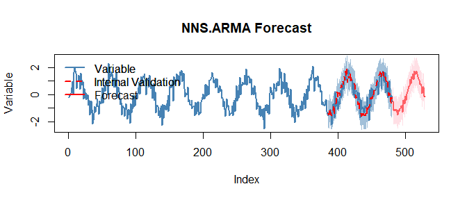

Figure 24.1. NNS.ARMA(..., h = 45, seasonal.factor = c(12,24,36)) forecast output with fitted trajectory and uncertainty structure.

24.10 Dynamic Updating and Recursive Forecast Paths

A one-step forecast is rarely the end goal. In practice, analysts often require

\[ h = 1,2,\dots,H \]

steps ahead.

In the NNS framework, multi-step forecasting proceeds recursively.

If \(\hat X_{T+1}\) is forecast first, then it is appended to the series and treated as part of the evolving path when forecasting \(\hat X_{T+2}\), and so on.

This creates two natural modes.

24.10.1 Static seasonal structure

The seasonal lags and weights are estimated once from the historical sample and then held fixed for all future steps.

24.10.2 Dynamic seasonal structure

The seasonal structure is recomputed as the forecast path grows, allowing the decomposition itself to evolve.

The static approach favors stability. The dynamic approach favors adaptability.

But that distinction can be made more precise.

Static updating is generally preferable when:

the dominant seasonal pattern is well known in advance,
the series is long enough that seasonal weights are already stable,
the forecast horizon is short relative to the seasonal period,
or the analyst values interpretability and reproducibility over rapid adaptation.

In such cases, recomputing the lag structure at every step may add noise rather than information. If the underlying periodic structure is persistent, then a fixed decomposition acts as a stabilizer.

Dynamic recomputation is preferable when the data suggest that the seasonal structure itself is moving. Typical signals include:

abrupt level shifts,
changing amplitudes of recurring cycles,
newly emerging or fading periodicities,
strong structural breaks,
or forecast errors that begin to cluster by phase.

For example, a retail series may historically be dominated by an annual pattern, yet after a major platform change or supply shock, shorter promotional cycles may become more predictive than the old annual rhythm. In that case, holding the original seasonal factor fixed can lock the forecast into an outdated regime. Dynamic updating allows the decomposition to respond as the series evolves.

So the practical decision is not merely “stability versus adaptability.” It is a question of whether the analyst believes the lag structure is itself part of the stable signal or part of the changing environment.

A useful empirical guide is out-of-sample validation. One may reserve a holdout period, compare static and dynamic forecasts over that window, and select the updating rule that yields better predictive accuracy. In that sense, the static-versus-dynamic decision is not purely philosophical. It can be treated as a forecasting design choice subject to cross-validation.

24.11 Prediction Intervals for Forecasts

Point forecasts are only one part of the forecasting problem. Analysts also need measures of uncertainty.

Because the NNS framework is nonparametric, forecast intervals are constructed without Gaussian error assumptions. Instead, uncertainty can be propagated using the maximum entropy bootstrap machinery developed in Chapter 17.

The logic is straightforward:

generate replicates consistent with the forecast path and dependence structure,
compute the implied distribution of future outcomes,
extract lower and upper predictive bounds from directional quantiles.

This produces prediction intervals that are aligned with the empirical distributional shape of the series rather than with a parametric error law.

Thus the directional framework provides not only nonlinear point forecasts, but also distribution-free forecast uncertainty quantification.

A bit more concretely, suppose the fitted model yields a forecast path

\[ \hat X_{T+1}, \dots, \hat X_{T+H}. \]

The bootstrap procedure does not assume i.i.d. Gaussian residuals around that path. Instead, it constructs synthetic continuations that preserve the rank structure and dependence features of the observed series as closely as possible. Each bootstrap replicate yields an alternative future trajectory, and the collection of such trajectories forms an empirical predictive distribution at each horizon.

If the series is asymmetric, heavy-tailed, or exhibits occasional bursts, those features can appear in the predictive distribution instead of being averaged away by a normal approximation. Directional lower and upper tail functionals can then be used to extract forecast bands. In this sense, the interval forecast is not an accessory to the point forecast. It is the distributional analogue of the same nonparametric logic: preserve the observed structure first, summarize uncertainty second.

In practice, one might generate a large number of bootstrap replicates, often on the order of hundreds or thousands, then evaluate the empirical future distribution at each horizon. If a central \(100(1-\alpha)\%\) interval is desired, the lower and upper bounds can be extracted from directional quantiles corresponding to \(\alpha/2\) and \(1-\alpha/2\). The exact number of replicates is an accuracy-versus-computation choice, but the principle is always the same: empirical resampled paths replace parametric error formulas.

24.12 Relation to Earlier NNS Chapters

Time-series modeling in NNS is not an isolated technique. It is a direct extension of earlier ideas.

24.12.1 From Chapter 18

The forecast engine is built from recursive conditional estimation.

24.12.2 From Chapter 19

The local regression on component series inherits the data-adaptive bandwidth logic of partition estimators.

24.12.3 From Chapter 21

Forecasting is just regression where the predictor is lagged time index or lagged structure and the response is the next component value.

24.12.4 From Chapter 23

Aggregation across multiple lag structures is an ensemble of directional learners.

So the time-series framework is not an exception to the book’s theory. It is one of its most natural applications.

24.13 Comparison with ARIMA

ARIMA remains one of the benchmark tools of time-series forecasting.

Its strengths are well known:

interpretable lag operators,
strong theory under stationarity,
effective performance on linear stochastic dynamics.

But its limitations are equally clear when viewed through the directional lens.

24.13.1 Structural form

ARIMA assumes a linear dependence structure after differencing. NNS does not.

24.13.2 Stationarity

ARIMA is built around stationarity and invertibility conditions. NNS forecasting does not require the series to satisfy a stationary parametric model in level.

24.13.3 Identification burden

ARIMA requires order selection and specification diagnostics. NNS shifts the task from parametric identification to predictive lag decomposition.

24.13.4 Nonlinearity

ARIMA can approximate some nonlinear behavior through transformations or hybridization, but nonlinearity is not native to the model. In NNS, it is native.

This does not mean ARIMA is obsolete. It means that ARIMA is best understood as a special, linear, tightly structured case of a broader forecasting problem.

For balance, however, NNS does not eliminate modeling choices. It replaces ARIMA’s order-identification problem with choices about lag selection, regression method, aggregation weights, and updating scheme. The difference is methodological rather than absolute: in NNS, these choices are naturally evaluated by predictive performance rather than by adherence to a pre-specified parametric identification protocol.

24.14 Comparison with ETS Models

ETS methods model time series through combinations of

error,
trend,
and seasonality,

typically using exponential smoothing recursions and state-space interpretations.

These methods are often highly effective, especially on business forecasting problems with stable level, trend, and seasonal components.

Relative to ETS, the NNS approach differs in several ways.

24.14.1 Component meaning

ETS decomposes the series into latent level, trend, and seasonality states. NNS decomposes it into lag-defined predictive subsets.

24.14.2 Smoothing mechanism

ETS uses recursive smoothing equations. NNS uses local regression and weighted aggregation across component series.

24.14.3 Parametric structure

ETS specifies an updating architecture in advance. NNS lets the predictive structure emerge from the data.

24.14.4 Nonlinear interactions

ETS can adapt smoothly, but it is not inherently designed for rich nonlinear autoregressive geometry. NNS is.

The practical difference is conceptual:

ETS smooths a presumed component architecture. NNS learns a predictive architecture from subset behavior.

A further distinction is distributional. Many ETS formulations are estimated in likelihood-based frameworks tied to specific error models, often Gaussian or close variants. The NNS approach imposes no such distributional law on the series or on the forecast errors.

24.15 When the NNS Approach Is Especially Useful

The nonparametric time-series framework is particularly attractive when one or more of the following hold:

the series exhibits nonlinear cyclic behavior,
multiple seasonalities are present,
model stationarity is doubtful,
lag effects are structurally asymmetric,
parametric identification is fragile,
or prediction accuracy matters more than adherence to a classical stochastic specification.

Examples include:

retail and transaction flows,
cyclical economic indicators,
energy demand,
financial and commodity time series,
and operational processes with threshold-driven dynamics.

These are precisely the settings where local structure matters more than global parametric elegance.

24.16 Limitations

A nonparametric forecasting method is not free of tradeoffs.

24.16.1 Primarily univariate in this chapter

The methods developed here focus on a single series. Cross-series interactions are deferred to Chapter 25.

24.16.2 Data requirements

Because prediction is learned from historical structure, sparse component series may limit reliability for very large lag lengths.

24.16.3 Computational cost

Searching many seasonal combinations and fitting nonlinear regressions can be more computationally intensive than fitting a simple linear ARIMA.

24.16.4 Interpretability of dynamics

A fitted ARIMA equation provides direct coefficients. NNS instead provides a predictive mechanism based on component regressions and weights. This is often more flexible, but less compact as a closed-form law.

These limitations are real. But they are the cost of avoiding the stronger assumptions of parametric time-series models.

The multivariate extension is natural in principle, but not automatic in implementation. Once several series enter, one must distinguish self-dependence from cross-dependence, align potentially different frequencies, and account for lead-lag structure across variables. Those complications motivate the next chapter.

24.17 Leakage-Safe Backtesting Protocol

Forecasting performance must be assessed with strict time-order preservation. A leakage-safe protocol is:

Rolling-origin evaluation: choose an initial training window [1, T_0].
Forecast horizon definition: for each origin t, produce forecasts for t+h without using observations after t.
Expanding or sliding refit:
- expanding window: train on [1, t], or
- sliding window: train on [t-w+1, t].
No future-informed preprocessing: any scaling, interpolation, imputation, or feature construction must be computed using data available at origin t only.
Horizon-specific scoring: report MAE/RMSE/coverage separately for each horizon h rather than pooling all horizons.
Interval calibration check: compare nominal vs empirical coverage for prediction intervals across horizons.

For seasonal component construction, lag selection must also be origin-specific; selecting global lags from the full sample before backtesting constitutes leakage.

24.18 Summary

This chapter developed nonparametric time-series modeling in the NNS framework.

Its main contributions are fivefold.

First, it reframed time series as a subset regression problem. Forecasting is treated as conditional estimation on lag-defined component series rather than as fitting a single global linear recursion.

Second, it developed seasonal decomposition by predictive concentration. Seasonal structure is detected through reductions in coefficient of variation across component series, linking seasonality directly to forecastability.

Third, it established nonlinear autoregressive forecasting. Component series are projected forward using nonparametric regression, allowing local curvature and asymmetric dynamics to enter the forecast natively.

Fourth, it clarified how the book’s broader dependence framework extends into time. Lagged directional structure can be studied theoretically through co-partial-moment ideas, even though the chapter’s main forecasting routines operationalize time dependence through component regression and seasonality rather than through a standalone directional-autocorrelation statistic.

Fifth, it clarified the chapter’s relationship to classical methods. ARIMA and ETS remain important special-purpose tools, but they impose structural assumptions that the NNS framework avoids.

Taken together, these results show that the directional nonparametric framework extends naturally from cross-sectional estimation to temporal prediction.

But the framework developed here remains fundamentally univariate. Once other series matter, the main difficulty is no longer just whether the past of \(X_t\) predicts its future, but whether lagged values of \(Y_t\), \(Z_t\), and other related processes alter that forecast in nonlinear and asymmetric ways. In that setting, univariate decomposition can miss cross-series lead-lag effects, common shocks, and mixed-frequency structure.

The next chapter therefore generalizes the same ideas to multivariate forecasting, where multiple time series interact through directional dependence, lagged cross-variable structure, and mixed-frequency information.

Further Reading / Examples For forecasting applications, including the tidal data example, see the NNS Time-Series Forecasting Examples. This behavior is illustrated in the tidal forecasting example, where the seasonal decomposition captures the dominant 12-month cycle.