Getting Started with NNS: Sampling and Simulation

library(NNS)
library(data.table)
require(knitr)
require(rgl)

NNS offers several novel sampling methods from any distribution, as well as simulating variables while maintaining their dependence.

Sampling

CDFs

Cumulative distribution functions (CDFs) represent the probability a variable $X$ will take a value less than or equal to $x$ . $F(x) = P(X \leq x)$

Empirical CDF

The empirical CDF is a simple construct, provided in the base package of R. We can generate an empirical CDF with the ecdf function and create a function (P) to return the CDF of a given value of $X$ .

set.seed(123); x = rnorm(100)
ecdf(x)

## Empirical CDF 
## Call: ecdf(x)
##  x[1:100] = -2.3092, -1.9666, -1.6867,  ...,  2.169, 2.1873

P = ecdf(x)
P(0); P(1)

## [1] 0.48

## [1] 0.83

Lower Partial Moment CDF (`LPM.ratio`)

The empirical CDF and Lower Partial Moment CDF (LPM.ratio) are identical when the degree term of the LPM.ratio is set to zero.

Degree 0 LPM: $LPM(0,t,X)=\frac{1}{N}\sum_{n=1}^{N}[max(t-X_n),0]^0$ LPM.ratio is equivalent to the following form for any target $(t)$ and variable $X$ : $LPM(0,t,X)=\frac{LPM(0,t,X)}{LPM(0,t,X)+UPM(0,t,X)}$

Using the same targets from our ecdf example above (0,1) we can compare LPM.ratios.

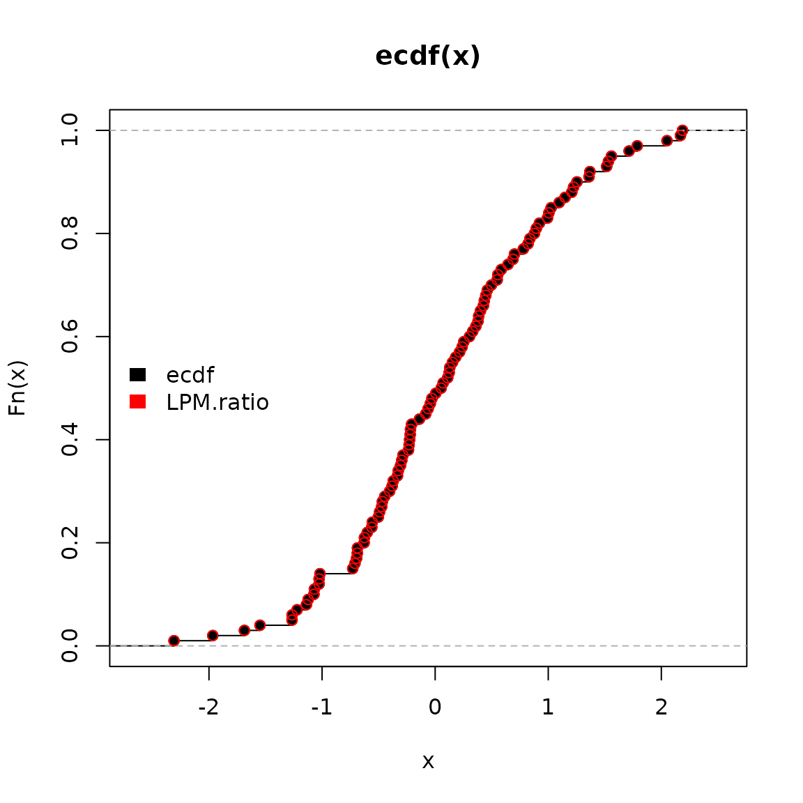
LPM.ratio(degree = 0, target = 0, variable = x); LPM.ratio(degree = 0, target = 1, variable = x)

## [1] 0.48

## [1] 0.83

Calculating the probability for every target value in $X$ , we can plot both methods visualizing their identical results. ecdf function in black and LPM.ratio in red.

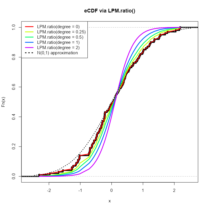
`LPM.ratio` degree > 0

By simply increasing the degree parameter to any positive real number, we can generate different CDFs of our initial distribution $x$ .

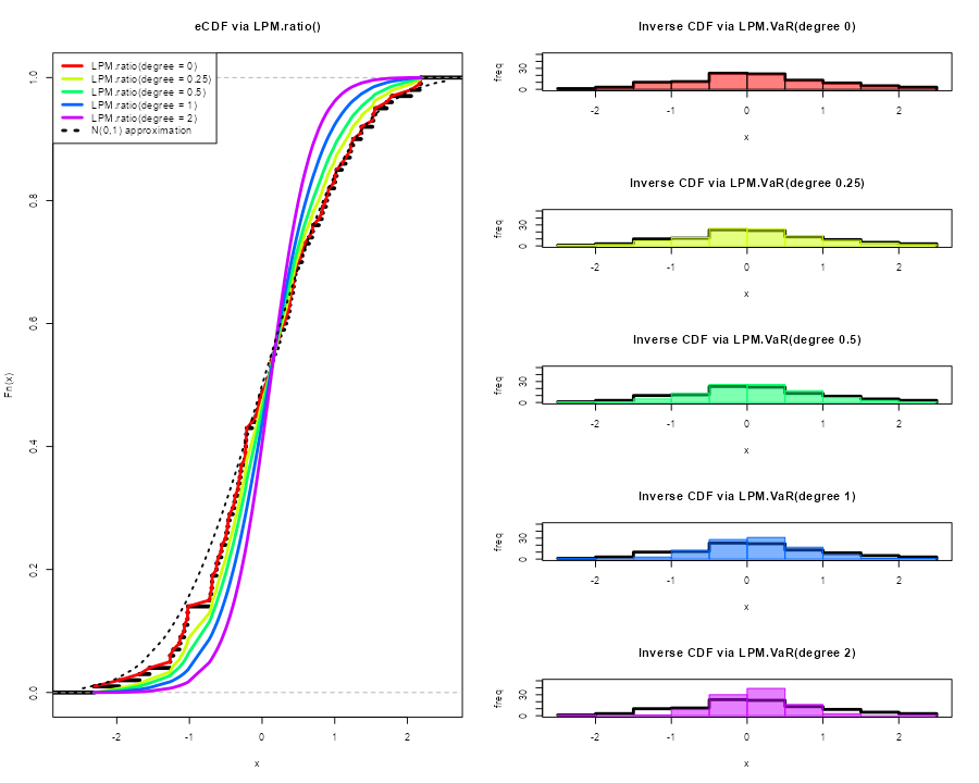
Generating PDFs with (`LPM.VaR`)

We can now generate distributions using the same insights and degree manipulation in the corresponding LPM.VaR function, a la value-at-risk, providing inverse CDF estimates.

The general form in the following plots is:

LPM.VaR(percentile = seq(0, 1, length.out = 100), degree = 0, x = x)

Any length percentile can be used to sample from the underlying distribution $x$ .

Viewing the first 10 samples from each of the degrees compared to our original $X$ .

degree.0.samples = LPM.VaR(percentile = seq(0, 1, length.out = 100), degree = 0, x = x)
degree.0.25.samples = LPM.VaR(percentile = seq(0, 1, length.out = 100), degree = 0.25, x = x)
degree.0.5.samples = LPM.VaR(percentile = seq(0, 1, length.out = 100), degree = 0.5, x = x)
degree.1.samples = LPM.VaR(percentile = seq(0, 1, length.out = 100), degree = 1, x = x)
degree.2.samples = LPM.VaR(percentile = seq(0, 1, length.out = 100), degree = 2, x = x)

head(data.table::data.table(cbind("original x" = sort(x), degree.0.samples, 
                                                          degree.0.25.samples, 
                                                          degree.0.5.samples, 
                                                          degree.1.samples, 
                                                          degree.2.samples)), 10)

     original x degree.0.samples degree.0.25.samples degree.0.5.samples
  1:  -2.309169        -2.309169           -2.309097         -2.3090915
  2:  -1.966617        -1.966617           -1.941190         -1.6935509
  3:  -1.686693        -1.686693           -1.599486         -1.4541494
  4:  -1.548753        -1.548753           -1.382553         -1.2462731
  5:  -1.265396        -1.265396           -1.250823         -1.1453748
  6:  -1.265061        -1.265061           -1.176436         -1.0745440
  7:  -1.220718        -1.220718           -1.119655         -1.0252742
  8:  -1.138137        -1.138137           -1.067793         -0.9868693
  9:  -1.123109        -1.123109           -1.026429         -0.9322105
 10:  -1.071791        -1.071791           -1.014276         -0.8710942
     degree.1.samples degree.2.samples
  1:       -2.3091021       -2.3091170
  2:       -1.4744653       -1.1614908
  3:       -1.2159961       -0.9709972
  4:       -1.0823023       -0.8610192
  5:       -0.9968028       -0.7810300
  6:       -0.9290505       -0.7169770
  7:       -0.8666886       -0.6631888
  8:       -0.8090433       -0.6170691
  9:       -0.7556644       -0.5765608
 10:       -0.7069835       -0.5403318

Simulation

Bootstrapping (`NNS.meboot`)

NNS.meboot is based on the maximum entropy bootstrap, available in the R-package meboot. This procedure is specifically designed for time-series and avoids the IID assumption in traditional methods.

The ability to sample from specified correlations ensures the full spectrum of future paths is sampled from. Typical Monte Carlo samples are restricted to [-0.3, 0.3] correlations to the original data.

We will generate 1 replicate of $X$ for each value of a sequence of $\rho$ values (the $ensemble$ ), and then plot the results compared to our original $X$ (black line). NNS.MC is a streamlined wrapper function for this functionality of NNS.meboot.

boots = NNS.MC(x, reps = 1, lower_rho = -1, upper_rho = 1, by = .5)$replicates
reps = do.call(cbind, boots)


matplot(reps, type = "l", col = rainbow(length(boots)))
lines(x, type = "l", lwd = 3, ylim = c(min(reps), max(reps)))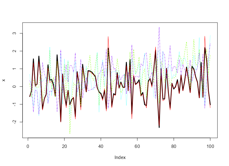

Checking our replicate correlations:

sapply(boots, function(r) cor(r, x, method = "spearman"))

    rho = 1   rho = 0.5     rho = 0  rho = -0.5    rho = -1 
 0.99732373  0.51147915  0.01036904 -0.48720072 -0.98294629

More replicates and ensembles thereof can be generated for any number of $\rho$ values.

`target_drift` Specification

We can also specify a target drift in our replicates with the target_drift parameter.

boots = NNS.MC(x, reps = 1, lower_rho = -1, upper_rho = 1, by = .5, target_drift = 0.05)$replicates
reps = do.call(cbind, boots)

plot(x, type = "l", lwd = 3, ylim = c(min(c(x, reps)), max(c(x, reps))))
matplot(reps, type = "l", col = rainbow(length(boots)), add = TRUE)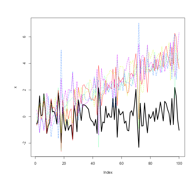

Please see the full NNS.meboot and NNS.MC argument documentation.

Simulating a Multivariate Dependence Structure

Analogous to an empirical copula transformation, we can generate new data from the dependence structure of our original data via the following steps:

Determine the dependence structure:

This is accomplished using LPM.ratio(1, x, x) for continuous variables, and LPM.ratio(0, x, x) for discrete variables, which are the empirical CDFs of the marginal variables.

Generate or supply new data:

new data does not have to be of the same distribution or dimension as the original data, nor does each dimension of new data have to share a distribution type.

Apply dependence structure to new data:

We then utilize LPM.VaR to ascertain new data values corresponding to original data position mappings, and return a matrix of these transformed values with the same dimensions as new.data.

set.seed(123)
x = rnorm(1000); y = rnorm(1000); z = rnorm(1000)

# Add variable x to original data to avoid total independence (example only)
original.data = cbind(x, y, z, x)

# Determine dependence structure
dep.structure = apply(original.data, 2, function(x) LPM.ratio(degree = 1, target = x, variable = x))
  
# Generate new data with different mean, sd and length (or distribution type)
new.data = sapply(1:ncol(original.data), function(x) rnorm(nrow(original.data)*2, mean = 10, sd = 20))

# Apply dependence structure to new data
new.dep.data = sapply(1:ncol(original.data), function(x) LPM.VaR(percentile = dep.structure[,x], degree = 1, x = new.data[,x]))

Compare Multivariate Dependence Structures

Similar dependence with radically different values, since we used $N(10, 20)$ in place of our original $N(0,1)$ observations.

NNS.copula(original.data)
NNS.copula(new.dep.data)

[1] 0.4743531
[1] 0.4753264

head(original.data)
head(new.dep.data)

               x           y          z           x
[1,] -0.56047565 -0.99579872 -0.5116037 -0.56047565
[2,] -0.23017749 -1.03995504  0.2369379 -0.23017749
[3,]  1.55870831 -0.01798024 -0.5415892  1.55870831
[4,]  0.07050839 -0.13217513  1.2192276  0.07050839
[5,]  0.12928774 -2.54934277  0.1741359  0.12928774
[6,]  1.71506499  1.04057346 -0.6152683  1.71506499
          [,1]       [,2]       [,3]      [,4]
[1,] -2.028109 -10.498044 -0.2090467 -1.682949
[2,]  4.608303 -11.390485 15.6213689  4.852534
[3,] 39.478741   8.836581 -0.8508203 40.585505
[4,] 10.683731   6.609255 36.0328589 10.877677
[5,] 11.866922 -47.955235 14.3111350 12.064633
[6,] 42.665726  29.639640 -2.4141874 43.797025

Alternative Using `NNS.meboot`

Alternatively, if we wish to keep the simulated values close to the original data, we can apply the NNS.meboot procedure to each of the variables.

We will generate 1 replicate (for brevity) of $\rho = 0.95$ to our original.data, use their ensemble and note the multivariate dependence among our new.boot.dep.data.

# Apply bootstrap to each variable
new.boot.dep.data = apply(original.data, 2, function(r) NNS.meboot(r, reps = 100, rho = .95))

# Reformat into vectors
boot.ensemble.vectors = lapply(new.boot.dep.data, function(z) unlist(z["ensemble",]))

# Create matrix from vectors
new.boot.dep.matrix = do.call(cbind, boot.ensemble.vectors)

Checking ensemble correlations with original.data:

for(i in 1:4) print(cor(new.boot.dep.matrix[,i], original.data[,i], method = "spearman"))

[1] 0.9452863
[1] 0.9499478
[1] 0.945878
[1] 0.9442845

Compare Multivariate Dependence Structures

Similar dependence with similar values.

NNS.copula(original.data)
NNS.copula(new.boot.dep.matrix)

[1] 0.4743531
[1] 0.4517661

head(original.data)
head(new.boot.dep.matrix)

               x           y          z           x
[1,] -0.56047565 -0.99579872 -0.5116037 -0.56047565
[2,] -0.23017749 -1.03995504  0.2369379 -0.23017749
[3,]  1.55870831 -0.01798024 -0.5415892  1.55870831
[4,]  0.07050839 -0.13217513  1.2192276  0.07050839
[5,]  0.12928774 -2.54934277  0.1741359  0.12928774
[6,]  1.71506499  1.04057346 -0.6152683  1.71506499
                   x          y          z          x
ensemble1 -0.4268047 -0.7794553 -0.6364458 -0.4642642
ensemble2 -0.2965744 -1.0682197  0.3297265 -0.2531178
ensemble3  1.3302149  0.3054734 -0.4014515  1.4914884
ensemble4  0.2257378  0.3108846  1.0603892  0.1728540
ensemble5  0.4716743 -3.3344967 -0.1917697  0.4309379
ensemble6  1.3984978  1.1881374 -0.5295386  1.5326055

References

If the user is so motivated, detailed arguments and proofs are provided within the following:

Fred Viole

Sampling

CDFs

Empirical CDF

Lower Partial Moment CDF (LPM.ratio)

LPM.ratio degree > 0

Generating PDFs with (LPM.VaR)

Simulation

Bootstrapping (NNS.meboot)

target_drift Specification

Simulating a Multivariate Dependence Structure

Compare Multivariate Dependence Structures

Alternative Using NNS.meboot

Compare Multivariate Dependence Structures

References

Lower Partial Moment CDF (`LPM.ratio`)

`LPM.ratio` degree > 0

Generating PDFs with (`LPM.VaR`)

Bootstrapping (`NNS.meboot`)

`target_drift` Specification

Alternative Using `NNS.meboot`