Getting Started with NNS: Overview

# Prereqs (uncomment if needed):
# install.packages("NNS")
# install.packages(c("data.table","xts","zoo","Rfast"))

library(NNS)

## Warning in rgl.init(initValue, onlyNULL): RGL: unable to open X11 display

## Warning: 'rgl.init' failed, will use the null device.
## See '?rgl.useNULL' for ways to avoid this warning.

library(data.table)

Orientation

Goal. A complete, hands‑on curriculum for Nonlinear Nonparametric Statistics (NNS) using partial moments. Each section blends narrative intuition, precise math, and executable code.

Structure.

Foundations — partial moments & variance decomposition
Descriptive & distributional tools
Dependence & nonlinear association
Hypothesis testing & ANOVA (LPM‑CDF)
Regression, boosting, stacking & causality
Time series & forecasting
Normalziation & Rescaling
Simulation (max‑entropy) & Monte Carlo
Portfolio & stochastic dominance

Notation. For a random variable $X$ and threshold/target $t$ , the population $n$ ‑th partial moments are defined as

$\operatorname{LPM}(n,t,X) = \int_{-\infty}^{t} (t-x)^{n} \, dF_X(x), \qquad \operatorname{UPM}(n,t,X) = \int_{t}^{\infty} (x-t)^{n} \, dF_X(x).$

The empirical estimators replace $F_X$ with the empirical CDF $\hat F_n$ (or, equivalently, use indicator functions):

$\widehat{\operatorname{LPM}}_n(t;X) = \frac{1}{n} \sum_{i=1}^n (t-x_i)^n \, \mathbf{1}_{\{x_i \le t\}}, \qquad \widehat{\operatorname{UPM}}_n(t;X) = \frac{1}{n} \sum_{i=1}^n (x_i-t)^n \, \mathbf{1}_{\{x_i > t\}}.$

These correspond to integrals over the measurable subsets $\{X \le t\}$ and $\{X > t\}$ in a $\sigma$ ‑algebra; the empirical sums are discrete analogues of Lebesgue integrals.

1. Foundations — Partial Moments & Variance Decomposition

1.1 Why partial moments

Classical variance treats upside and downside symmetrically. Partial moments separate them, allowing asymmetric risk/reward analysis around a chosen target $t$ (often the mean or a benchmark).
At $t=\mu_X$ : $\operatorname{Var}(X) = \operatorname{UPM}(2,\mu_X,X) + \operatorname{LPM}(2,\mu_X,X)\quad\text{(exact empirical identity)}.$ This is not the same as splitting conditional variances around a threshold; partial moments use a global reference, preserving the between‑group contribution.

1.2 Core functions and headers

LPM(degree, target, variable)
UPM(degree, target, variable)

1.3 Code: variance decomposition & CDF

set.seed(42)

# Normal sample
y <- rnorm(3000)
mu <- mean(y)
L2 <- LPM(2, mu, y); U2 <- UPM(2, mu, y)
cat(sprintf("LPM2 + UPM2 = %.6f vs var(y)=%.6f\n", (L2+U2)*(length(y) / (length(y) - 1)), var(y)))

## LPM2 + UPM2 = 1.011889 vs var(y)=1.011889

# Empirical CDF via LPM.ratio(0, t, x)
for (t in c(-1,0,1)) {
  cdf_lpm <- LPM.ratio(0, t, y)
  cat(sprintf("CDF at t=%+.1f : LPM.ratio=%.4f | empirical=%.4f\n", t, cdf_lpm, mean(y<=t)))
}

## CDF at t=-1.0 : LPM.ratio=0.1633 | empirical=0.1633
## CDF at t=+0.0 : LPM.ratio=0.5043 | empirical=0.5043
## CDF at t=+1.0 : LPM.ratio=0.8480 | empirical=0.8480

# Asymmetry on a skewed distribution
z <- rexp(3000)-1; mu_z <- mean(z)
cat(sprintf("Skewed z: LPM2=%.4f, UPM2=%.4f (expect imbalance)\n", LPM(2,mu_z,z), UPM(2,mu_z,z)))

## Skewed z: LPM2=0.2780, UPM2=0.7682 (expect imbalance)

Interpretation. The equality LPM2 + UPM2 == var(x) (Bessel adjustment used) holds because deviations are measured against the global mean. LPM.ratio(0, t, x) constructs an empirical CDF directly from partial‑moment counts.

2. Descriptive & Distributional Tools

2.1 Higher moments from partial moments

Define asymmetric analogues of skewness/kurtosis using $\operatorname{UPM}_3$ , $\operatorname{LPM}_3$ (and degree 4), yielding robust tail diagnostics without parametric assumptions.

Header. NNS.moments(x)

M <- NNS.moments(y)
M

## $mean
## [1] -0.0114498
## 
## $variance
## [1] 1.011552
## 
## $skewness
## [1] -0.007412142
## 
## $kurtosis
## [1] 0.06723772

2.2 Mode estimation (no bin‑or‑bandwidth angst)

Header. NNS.mode(x)

set.seed(23)
multimodal <- c(rnorm(1500,-2,.5), rnorm(1500,2,.5))
NNS.mode(multimodal,multi = TRUE)

## [1] -2.049405  1.987674

2.3 CDF tables via LPM ratios

Headers.

LPM.ratio(degree = 0, target, variable) (empirical CDF when degree=0)
UPM.ratio(degree = 0, target, variable)
LPM.VaR(p, degree, variable) (quantiles via partial‑moment CDFs)
UPM.VaR(p, degree, variable)

qgrid <- LPM.VaR(seq(0.05,0.95,.1),0,z) # equivalent to quantile(z,probs = seq(0.05,0.95,by=0.1))
CDF_tbl <- data.table(threshold = as.numeric(qgrid), CDF = LPM.ratio(0,qgrid,z))
CDF_tbl

##       threshold   CDF
##           <num> <num>
##  1: -0.94052127  0.05
##  2: -0.83748109  0.15
##  3: -0.71317882  0.25
##  4: -0.57443327  0.35
##  5: -0.41017671  0.45
##  6: -0.20424962  0.55
##  7:  0.06850182  0.65
##  8:  0.41462712  0.75
##  9:  0.94307172  0.85
## 10:  2.09633977  0.95

3. Dependence & Nonlinear Association

3.1 Why move beyond Pearson $r$

Pearson captures linear monotone relationships. Many structures (U‑shapes, saturation, asymmetric tails) produce near‑zero $r$ despite strong dependence. Partial‑moment dependence metrics respond to such structure.

Headers.

Co.LPM(degree_lpm, x, y, target_x, target_y, degree_y) / Co.UPM(...) (co‑partial moments)
PM.matrix(LPM_degree, UPM_degree, target=NULL, variable, pop_adj=TRUE)
NNS.dep(x, y) (scalar dependence coefficient)
NNS.copula(X, target=NULL, continuous=TRUE, plot=FALSE, independence.overlay=FALSE)

3.2 Code: nonlinear dependence

set.seed(1)
x <- runif(2000,-1,1)
y <- x^2 + rnorm(2000, sd=.05)
cat(sprintf("Pearson r = %.4f\n", cor(x,y)))

## Pearson r = 0.0006

cat(sprintf("NNS.dep  = %.4f\n", NNS.dep(x,y)$Dependence))

## NNS.dep  = 0.7097

X <- data.frame(a=x, b=y, c=x*y + rnorm(2000, sd=.05))
pm <- PM.matrix(1, 1, target = "means", variable=X, pop_adj=TRUE)
pm

## $cupm
##            a          b          c
## a 0.17384174 0.05668152 0.10450858
## b 0.05668152 0.05566363 0.04414923
## c 0.10450858 0.04414923 0.07529373
## 
## $dupm
##              a          b            c
## a 0.0000000000 0.05675501 0.0005598221
## b 0.0143108307 0.00000000 0.0036839026
## c 0.0004239566 0.04430691 0.0000000000
## 
## $dlpm
##              a           b            c
## a 0.0000000000 0.014310831 0.0004239566
## b 0.0567550147 0.000000000 0.0443069142
## c 0.0005598221 0.003683903 0.0000000000
## 
## $clpm
##            a           b           c
## a 0.16803827 0.014485430 0.102709867
## b 0.01448543 0.037120650 0.003051617
## c 0.10270987 0.003051617 0.074865823
## 
## $cov.matrix
##              a             b            c
## a 0.3418800141  0.0001011068  0.206234664
## b 0.0001011068  0.0927842833 -0.000789973
## c 0.2062346637 -0.0007899730  0.150159552

cop <- NNS.copula(X, continuous=TRUE, plot=FALSE)
cop

## [1] 0.5692785

3.3 Code: copula

# Data
set.seed(123); x = rnorm(100); y = rnorm(100); z = expand.grid(x, y)

# Plot
rgl::plot3d(z[,1], z[,2], Co.LPM(0, z[,1], z[,2], z[,1], z[,2]), col = "red")

# Uniform values
u_x = LPM.ratio(0, x, x); u_y = LPM.ratio(0, y, y); z = expand.grid(u_x, u_y)

# Plot
rgl::plot3d(z[,1], z[,2], Co.LPM(0, z[,1], z[,2], z[,1], z[,2]), col = "blue")

Interpretation. NNS.dep remains high for curved relationships; PM.matrix collects co‑partial moments across variables; NNS.copula summarizes higher‑dimensional dependence using partial‑moment ratios. Copulas are returned and evaluated via Co.LPM functions.

4. Normalization and Rescaling

NNS provides two main tools for scaling data while preserving rank structure and distributional shape. Both operate via deterministic affine transformations.

4.1 Normalization

NNS.norm() rescales variables to a common magnitude while preserving distributional structure. The method can be linear (all variables forced to have the same mean) or nonlinear (using dependence weights to produce a more nuanced scaling). In the nonlinear case, the degree of association between variables influences the final normalized values.

Header.

NNS.norm(x, linear=TRUE, chart.type = NULL)

A <- rnorm(100, mean = 0, sd = 1)
B <- rnorm(100, mean = 0, sd = 5)
C <- rnorm(100, mean = 10, sd = 1)
D <- rnorm(100, mean = 10, sd = 10)

X <- data.frame(A, B, C, D)

# Linear scaling
lin_norm <- NNS.norm(X, linear = TRUE, chart.type=NULL, location=NULL)

Interpretation. NNS.norm() brings variables to a common scale without distorting their distributional shape. Linear mode equalizes means; nonlinear mode additionally weights each variable by its dependence with others, so more correlated variables exert greater influence on the final scaling.

4.2 Risk‑neutral rescale (pricing context)

NNS.rescale() performs one‑dimensional affine transformations.

Header.

NNS.rescale(x, a, b, method=c("minmax","riskneutral"), T=NULL, type=c("Terminal","Discounted"))

px <- 100 + cumsum(rnorm(260, sd = 1))
rn <- NNS.rescale(px, a=100, b=0.03, method="riskneutral", T=1, type="Terminal")
c( target = 100*exp(0.03*1), mean_rn = mean(rn) )

##   target  mean_rn 
## 103.0455 103.0455

Interpretation. riskneutral shifts the mean to match $S_0 e^{rT}$ (Terminal) or $S_0$ (Discounted), preserving distributional shape.

5. Hypothesis Testing & ANOVA (LPM‑CDF)

5.1 Concept

Instead of distributional assumptions, compare groups via LPM‑based CDFs. Output is a degree of certainty (not a p‑value) for equality of populations or means.

Header.

NNS.ANOVA(control, treatment, means.only=FALSE, medians=FALSE, confidence.interval=.95, tails=c("Both","left","right"), pairwise=FALSE, plot=TRUE, robust=FALSE)

5.2 Code: two‑sample & multi‑group

ctrl <- rnorm(200, 0, 1)
trt  <- rnorm(180, 0.35, 1.2)
NNS.ANOVA(control=ctrl, treatment=trt, means.only=FALSE, plot=FALSE)

## $Control
## [1] 0.05568255
## 
## $Treatment
## [1] 0.2771257
## 
## $Grand_Statistic
## [1] 0.1605767
## 
## $Control_CDF
## [1] 0.5670595
## 
## $Treatment_CDF
## [1] 0.4385169
## 
## $Certainty
## [1] 0.6905166
## 
## $Effect_Size_LB
##        2.5% 
## -0.07055716 
## 
## $Effect_Size_UB
##     97.5% 
## 0.5317766 
## 
## $Confidence_Level
## [1] 0.95

A <- list(g1=rnorm(150,0.0,1.1), g2=rnorm(150,0.2,1.0), g3=rnorm(150,-0.1,0.9))
NNS.ANOVA(control=A, means.only=TRUE, plot=FALSE)

## Certainty 
## 0.6876008

Math sketch. For each quantile/threshold $t$ , compare CDFs built from LPM.ratio(0, t, •) (possibly with one‑sided tails). Aggregate across $t$ to a certainty score.

6. Regression, Boosting, Stacking & Causality

6.1 Philosophy

NNS.reg learns partitioned relationships using partial‑moment weights — linear where appropriate, nonlinear where needed — avoiding fragile global parametric forms.

Headers.

NNS.reg(x, y, order=NULL, smooth=TRUE, ncores=1, ...) → $Fitted.xy, $Point.est, …
NNS.boost(IVs.train, DV.train, IVs.test, epochs, learner.trials, status, balance, type, folds)
NNS.stack(IVs.train, DV.train, IVs.test, type, balance, ncores, folds)
NNS.caus(x, y) (directional causality score via conditional dependence)

6.2 Code: classification via regression + ensembles

# Example 1: Nonlinear regression
set.seed(123)
x_train <- runif(1000, -2, 2)
y_train <- sin(pi * x_train) + rnorm(1000, sd = 0.2)

x_test <- seq(-2, 2, length.out = 100)

NNS.reg(x = x_train, y = y_train, order = NULL, point.est = x_test)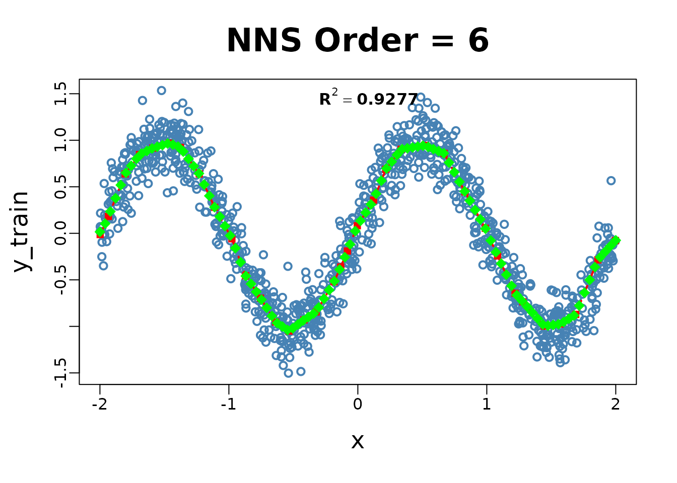

## $R2
## [1] 0.9276761
## 
## $SE
## [1] 0.2015258
## 
## $Prediction.Accuracy
## NULL
## 
## $equation
## NULL
## 
## $x.star
## NULL
## 
## $derivative
##     Coefficient X.Lower.Range X.Upper.Range
##           <num>         <num>         <num>
##  1:   3.0485215  -1.998138604  -1.934370540
##  2:   3.5169373  -1.934370540  -1.804387149
##  3:   1.8605016  -1.804387149  -1.692769075
##  4:   0.6783073  -1.692769075  -1.590915710
##  5:   0.4272848  -1.590915710  -1.465816449
##  6:  -0.5144026  -1.465816449  -1.376464546
##  7:  -1.9381128  -1.376464546  -1.229726997
##  8:  -3.0106084  -1.229726997  -1.110428636
##  9:  -2.5210796  -1.110428636  -0.976623793
## 10:  -3.7347021  -0.976623793  -0.870193992
## 11:  -2.0861598  -0.870193992  -0.754706576
## 12:  -2.1796417  -0.754706576  -0.636846031
## 13:  -0.9300308  -0.636846031  -0.533099369
## 14:   1.0359249  -0.533099369  -0.417818767
## 15:   0.9115004  -0.417818767  -0.323764665
## 16:   2.3250859  -0.323764665  -0.184330858
## 17:   3.0769180  -0.184330858  -0.132632209
## 18:   3.3162510  -0.132632209  -0.080933560
## 19:   3.5323950  -0.080933560  -0.004108338
## 20:   2.1862481  -0.004108338   0.121863569
## 21:   3.4805229   0.121863569   0.216987038
## 22:   1.8001452   0.216987038   0.336388996
## 23:   0.2295375   0.336388996   0.516729182
## 24:  -0.5625172   0.516729182   0.668479078
## 25:  -2.5532272   0.668479078   0.830264570
## 26:  -2.4765129   0.830264570   0.988320504
## 27:  -3.1248612   0.988320504   1.083380900
## 28:  -2.9622550   1.083380900   1.218812429
## 29:  -1.5047059   1.218812429   1.279773569
## 30:  -1.5723118   1.279773569   1.445979675
## 31:   0.1804598   1.445979675   1.571628940
## 32:   0.8726461   1.571628940   1.689536565
## 33:   3.4198918   1.689536565   1.860999223
## 34:   1.5206901   1.860999223   1.997618112
##     Coefficient X.Lower.Range X.Upper.Range
##           <num>         <num>         <num>
## 
## $Point.est
##   [1]  0.01571202  0.10442684  0.23470933  0.37680781  0.51890629  0.65039140
##   [7]  0.72556318  0.80073496  0.85698998  0.88439634  0.91180269  0.93033285
##  [13]  0.94759688  0.96486091  0.95248720  0.93170326  0.87827479  0.79996720
##  [19]  0.72165961  0.64335202  0.52449573  0.40285499  0.28121424  0.17901835
##  [25]  0.07715655 -0.02470525 -0.15949123 -0.31038828 -0.45880078 -0.54309006
##  [31] -0.62737935 -0.71234468 -0.80041101 -0.88847734 -0.96331853 -1.00089554
##  [37] -1.03847254 -1.02090671 -0.97905116 -0.93719561 -0.89956805 -0.86273975
##  [43] -0.79660165 -0.70265879 -0.60871593 -0.51288396 -0.38856404 -0.25667590
##  [49] -0.11829230  0.02443074  0.13442845  0.22276171  0.31109496  0.42473203
##  [55]  0.56535922  0.69718932  0.76992246  0.84265560  0.90432326  0.91359751
##  [61]  0.92287175  0.93214599  0.94142023  0.92794242  0.90521445  0.88248648
##  [67]  0.85975852  0.76020581  0.65704511  0.55388442  0.45072372  0.35051056
##  [73]  0.25044944  0.15038831  0.04930377 -0.07695325 -0.20321027 -0.32495818
##  [79] -0.44464525 -0.56433232 -0.66432673 -0.72512293 -0.78817431 -0.85170206
##  [85] -0.91522981 -0.97875756 -0.99186193 -0.98457062 -0.97727932 -0.95314667
##  [91] -0.91788824 -0.88262981 -0.77697785 -0.63880041 -0.50062296 -0.36244551
##  [97] -0.25805231 -0.19661029 -0.13516826 -0.07526941
## 
## $pred.int
## NULL
## 
## $regression.points
##                x           y
##            <num>       <num>
##  1: -1.998138604 -0.01307124
##  2: -1.934370540  0.18132707
##  3: -1.804387149  0.63847051
##  4: -1.692769075  0.84613612
##  5: -1.590915710  0.91522399
##  6: -1.465816449  0.96867700
##  7: -1.376464546  0.92271416
##  8: -1.229726997  0.63832023
##  9: -1.110428636  0.27915958
## 10: -0.976623793 -0.05817308
## 11: -0.870193992 -0.45565668
## 12: -0.754706576 -0.69658188
## 13: -0.636846031 -0.95347564
## 14: -0.533099369 -1.04996323
## 15: -0.417818767 -0.93054118
## 16: -0.323764665 -0.84481083
## 17: -0.184330858 -0.52061525
## 18: -0.132632209 -0.36154275
## 19: -0.080933560 -0.19009705
## 20: -0.004108338  0.08127998
## 21:  0.121863569  0.35668582
## 22:  0.216987038  0.68776523
## 23:  0.336388996  0.90270609
## 24:  0.516729182  0.94410093
## 25:  0.668479078  0.85873901
## 26:  0.830264570  0.44566388
## 27:  0.988320504  0.05423632
## 28:  1.083380900 -0.24281423
## 29:  1.218812429 -0.64399694
## 30:  1.279773569 -0.73572553
## 31:  1.445979675 -0.99705336
## 32:  1.571628940 -0.97437872
## 33:  1.689536565 -0.87148709
## 34:  1.860999223 -0.28510334
## 35:  1.997618112 -0.07734835
##                x           y
##            <num>       <num>
## 
## $Fitted.xy
##                x          y      y.hat  NNS.ID   gradient    residuals
##            <num>      <num>      <num>  <char>      <num>        <num>
##    1: -0.8496899 -0.5752368 -0.4984314 q121122 -2.0861598  0.076805376
##    2:  1.1532205 -0.6617217 -0.4496971 q221122 -2.9622550  0.212024652
##    3: -0.3640923 -0.7048691 -0.8815695 q122122  0.9115004 -0.176700402
##    4:  1.5320696 -0.8447168 -0.9815176 q222121  0.1804598 -0.136800802
##    5:  1.7618691 -0.9820881 -0.6241175 q222212  3.4198918  0.357970569
##   ---                                                                 
##  996:  1.3184955 -0.7988901 -0.7966085 q221222 -1.5723118  0.002281548
##  997:  0.5684553  1.1554781  0.9150041 q212122 -0.5625172 -0.240473993
##  998: -0.4340050 -0.7748325 -0.9473089 q122121  1.0359249 -0.172476359
##  999:  0.8383194  0.7041960  0.4257159 q212222 -2.4765129 -0.278480031
## 1000: -1.5647037  0.9467853  0.9264240 q111222  0.4272848 -0.020361366
##       standard.errors
##                 <num>
##    1:       0.1769692
##    2:       0.1783713
##    3:       0.1905081
##    4:       0.2044300
##    5:       0.2636784
##   ---                
##  996:       0.1971693
##  997:       0.2137362
##  998:       0.1831159
##  999:       0.2108312
## 1000:       0.2078031

# Simple train/test for boosting & stacking
test.set = 141:150
 
boost <- NNS.boost(IVs.train = iris[-test.set, 1:4], 
              DV.train = iris[-test.set, 5],
              IVs.test = iris[test.set, 1:4],
              epochs = 10, learner.trials = 10, 
              status = FALSE, balance = TRUE,
              type = "CLASS", folds = 5)


mean(boost$results == as.numeric(iris[test.set,5]))
[1] 1


boost$feature.weights; boost$feature.frequency

stacked <- NNS.stack(IVs.train = iris[-test.set, 1:4], 
                     DV.train = iris[-test.set, 5],
                     IVs.test = iris[test.set, 1:4],
                     type = "CLASS", balance = TRUE,
                     ncores = 1, folds = 1)
mean(stacked$stack == as.numeric(iris[test.set,5]))
[1] 1

6.3 Code: directional causality

NNS.caus(mtcars$hp,  mtcars$mpg)  # hp -> mpg

## Causation.x.given.y Causation.y.given.x           C(x--->y) 
##           0.2607148           0.3863580           0.3933374

NNS.caus(mtcars$mpg, mtcars$hp)   # hp -> mpg

## Causation.x.given.y Causation.y.given.x           C(y--->x) 
##           0.3863580           0.2607148           0.3933374

Interpretation. Examine asymmetry in scores to infer direction. The method conditions partial‑moment dependence on candidate drivers.

7. Time Series & Forecasting

Headers.

NNS.ARMA
NNS.ARMA.optim
NNS.seas
NNS.VAR

# Univariate nonlinear ARMA
z <- as.numeric(scale(sin(1:480/8) + rnorm(480, sd=.35)))

# Seasonality detection (prints a summary)
seasonal_period <- NNS.seas(z, plot = FALSE)
head(seasonal_period$all.periods)

##   Period Coefficient.of.Variation Variable.Coefficient.of.Variation
## 1    200                0.4267885                      8.540159e+16
## 2     96                0.4425880                      8.540159e+16
## 3     49                0.4615546                      8.540159e+16
## 4    198                0.4812956                      8.540159e+16
## 5    199                0.4885608                      8.540159e+16
## 6    146                0.4901054                      8.540159e+16

# Validate seasonal periods
NNS.ARMA.optim(z, h = 48, seasonal.factor = seasonal_period$periods, plot = TRUE, ncores = 1)

## [1] "CURRNET METHOD: lin"
## [1] "COPY LATEST PARAMETERS DIRECTLY FOR NNS.ARMA() IF ERROR:"
## [1] "NNS.ARMA(... method =  'lin' , seasonal.factor =  c( 51 ) ...)"
## [1] "CURRENT lin OBJECTIVE FUNCTION = 0.398327414917885"
## [1] "BEST method = 'lin', seasonal.factor = c( 51 )"
## [1] "BEST lin OBJECTIVE FUNCTION = 0.398327414917885"
## [1] "CURRNET METHOD: nonlin"
## [1] "COPY LATEST PARAMETERS DIRECTLY FOR NNS.ARMA() IF ERROR:"
## [1] "NNS.ARMA(... method =  'nonlin' , seasonal.factor =  c( 51 ) ...)"
## [1] "CURRENT nonlin OBJECTIVE FUNCTION = 2.75408671013046"
## [1] "BEST method = 'nonlin' PATH MEMBER = c( 51 )"
## [1] "BEST nonlin OBJECTIVE FUNCTION = 2.75408671013046"
## [1] "CURRNET METHOD: both"
## [1] "COPY LATEST PARAMETERS DIRECTLY FOR NNS.ARMA() IF ERROR:"
## [1] "NNS.ARMA(... method =  'both' , seasonal.factor =  c( 51 ) ...)"
## [1] "CURRENT both OBJECTIVE FUNCTION = 0.778172239627562"
## [1] "BEST method = 'both' PATH MEMBER = c( 51 )"
## [1] "BEST both OBJECTIVE FUNCTION = 0.778172239627562"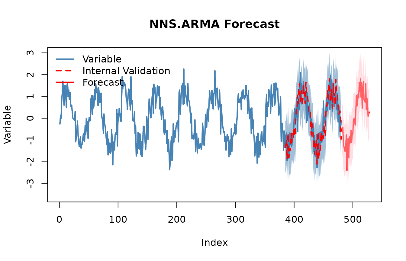

## $periods
## [1] 51
## 
## $weights
## NULL
## 
## $obj.fn
## [1] 0.3983274
## 
## $method
## [1] "lin"
## 
## $shrink
## [1] FALSE
## 
## $nns.regress
## [1] FALSE
## 
## $bias.shift
## [1] 0.01738357
## 
## $errors
##  [1] -0.4754897523 -0.4609730867 -0.3018876142  0.0439513384 -0.1128600832
##  [6]  0.9193835234  0.0160010547 -0.7516578805 -0.8195384972 -0.1274709629
## [11] -0.0093477175  0.1480424491  0.0345888303  0.0009331215 -0.2819915138
## [16] -0.3474821395 -1.2543849202 -0.5442948705 -0.0049610072 -0.4702036102
## [21]  0.1846614137  1.6541950586 -0.2046795992  0.9691745476  1.1460606178
## [26] -0.5141738440 -1.3562787956  0.3853973272 -0.3364881552 -0.5604890777
## [31] -0.3175309175 -0.1677932189 -0.1511705981  0.4541183441 -0.1377055180
## [36]  0.4279932502  1.3576081283 -0.0645315976  1.1430476887  0.1399600873
## [41]  0.0874395694 -0.3703494531  0.3046994756  0.2057574931 -0.7602832912
## [46]  0.6902933417  0.2238850985 -0.2775974238 -0.8250763050  0.5817787408
## [51] -0.8733350647  0.2906911996  0.1863210948 -0.2484232855  0.1444232735
## [56]  1.1655644133  0.0821221969 -0.2813315730 -0.7959981329 -0.3601165470
## [61] -0.4617740020 -0.0593491905  0.0143389607  0.1016580238  0.0300275332
## [66] -1.7237406556 -0.0930802461 -0.9348574200 -0.7189682901  0.0700766333
## [71] -0.3547205444  0.2333233909  0.6840012123 -0.0779445509  0.8409902584
## [76]  0.0130711684  0.8074727217 -1.1462424589  0.0926963526 -0.4674150054
## [81]  0.1308248298 -0.6493713604  0.0713668583  0.4889233461  0.4293197750
## [86] -0.4397639878  0.4261287370  0.7556075116  0.6016698079 -0.1086690282
## [91]  0.6426872057 -0.4175612763  0.0250816728  0.9344147185  0.5444153587
## [96] -0.8746369897
## 
## $results
##  [1] -0.495145166 -0.629911085 -0.423647703 -1.217211533 -1.313660334
##  [6] -1.507558621 -1.512809568 -1.244102492 -0.765300445 -2.402307464
## [11] -1.325990243 -0.928756118 -1.819067479 -0.855732188 -1.152690586
## [16] -1.039006594 -0.562011496 -1.103503510 -0.685097085 -0.727417601
## [21] -0.044018500 -0.030435409  0.002633325 -0.314902491  0.232587264
## [26]  1.030889038  0.556722546  0.680351082  1.101193382  0.941245213
## [31]  1.648626820  1.225992916  1.806473740  0.964372963  1.627354696
## [36]  0.460925955  1.318674310  1.692295367  0.854538440  0.768654797
## [41]  0.739228654  1.582319086  0.402156303  0.902802567  0.718513288
## [46]  0.086635865  0.193748286  0.283357285
## 
## $lower.pred.int
##  [1] -1.67077922 -1.80554514 -1.59928176 -2.39284559 -2.48929439 -2.68319268
##  [7] -2.68844363 -2.41973655 -1.94093450 -3.57794152 -2.50162430 -2.10439018
## [13] -2.99470154 -2.03136624 -2.32832464 -2.21464065 -1.73764555 -2.27913757
## [19] -1.86073114 -1.90305166 -1.21965256 -1.20606947 -1.17300073 -1.49053655
## [25] -0.94304679 -0.14474502 -0.61891151 -0.49528298 -0.07444068 -0.23438884
## [31]  0.47299276  0.05035886  0.63083968 -0.21126109  0.45172064 -0.71470810
## [37]  0.14304025  0.51666131 -0.32109562 -0.40697926 -0.43640540  0.40668503
## [43] -0.77347775 -0.27283149 -0.45712077 -1.08899819 -0.98188577 -0.89227677
## 
## $upper.pred.int
##  [1]  0.68048889  0.54572297  0.75198635 -0.04157748 -0.13802628 -0.33192456
##  [7] -0.33717551 -0.06846843  0.41033361 -1.22667341 -0.15035619  0.24687794
## [13] -0.64343342  0.31990187  0.02294347  0.13662746  0.61362256  0.07213055
## [19]  0.49053697  0.44821646  1.13161556  1.14519865  1.17826738  0.86073157
## [25]  1.40822132  2.20652310  1.73235660  1.85598514  2.27682744  2.11687927
## [31]  2.82426088  2.40162697  2.98210780  2.14000702  2.80298875  1.63656001
## [37]  2.49430837  2.86792942  2.03017250  1.94428885  1.91486271  2.75795314
## [43]  1.57779036  2.07843662  1.89414735  1.26226992  1.36938234  1.45899134

Notes. NNS seasonality uses coefficient of variation instead of ACF/PACFs, and NNS ARMA blends multiple seasonal periods into the linear or nonlinear regression forecasts.

8. Simulation & Bootstrap & Risk‑Neutral Rescaling

8.1 Maximum entropy bootstrap (shape‑preserving)

Header.

NNS.meboot(x, reps=999, rho=NULL, type="spearman", drift=TRUE, ...)

x_ts <- cumsum(rnorm(350, sd=.7))
mb <- NNS.meboot(x_ts, reps=5, rho = 1)
dim(mb["replicates", ]$replicates)

## [1] 350   5

8.2 Monte Carlo over the full correlation space

Header.

NNS.MC(x, reps=30, lower_rho=-1, upper_rho=1, by=.01, exp=1, type="spearman", ...)

mc <- NNS.MC(x_ts, reps=5, lower_rho=-1, upper_rho=1, by=.5, exp=1)
length(mc$ensemble); names(mc$replicates)

## [1] 350

## [1] "rho = 1"    "rho = 0.5"  "rho = 0"    "rho = -0.5" "rho = -1"

head(mc$replicates$`rho = 0`)

##      Replicate 1 Replicate 2 Replicate 3 Replicate 4 Replicate 5
## [1,]    8.561720   11.097841   12.140974    3.478574    16.25845
## [2,]    4.989649    9.142348    6.298598    2.573488    11.23749
## [3,]    5.489892   11.635826    9.151404    4.146175    13.61840
## [4,]    7.175210   13.194315   11.614209    5.906763    19.23707
## [5,]    8.443500   12.157572   13.263425    4.369562    13.40513
## [6,]    7.386515   10.979258   11.705842    2.410838    15.31133

9. Portfolio & Stochastic Dominance

Stochastic dominance orders uncertain prospects for broad classes of risk‑averse utilities; partial moments supply practical, nonparametric estimators.

Headers.

NNS.FSD.uni(x, y)
NNS.SSD.uni(x, y)
NNS.TSD.uni(x, y)
NNS.SD.cluster(R)
NNS.SD.efficient.set(R)

RA <- rnorm(240, 0.005, 0.03)
RB <- rnorm(240, 0.003, 0.02)
RC <- rnorm(240, 0.006, 0.04)

NNS.FSD.uni(RA, RB)

## [1] 0

NNS.SSD.uni(RA, RB)

## [1] 0

NNS.TSD.uni(RA, RB)

## [1] 0

Rmat <- cbind(A=RA, B=RB, C=RC)
try(NNS.SD.cluster(Rmat, degree = 1))

## $Clusters
## $Clusters$Cluster_1
## [1] "C" "A" "B"

try(NNS.SD.efficient.set(Rmat, degree = 1))

## Checking 1 of 2Checking 2 of 2

## [1] "C" "A" "B"

Appendix A — Measure‑theoretic sketch (why partial moments are rigorous)

Let $(\Omega, \mathcal{F}, \mathbb{P})$ be a probability space, $X: \Omega\to\mathbb{R}$ measurable. For any fixed $t\in\mathbb{R}$ , the sets $\{X\le t\}$ and $\{X>t\}$ are in $\mathcal{F}$ because they are preimages of Borel sets. The population partial moments are

$\operatorname{LPM}(k,t,X) = \int_{-\infty}^{t} (t-x)^k\, dF_X(x), \qquad \operatorname{UPM}(k,t,X) = \int_{t}^{\infty} (x-t)^k\, dF_X(x).$

The empirical versions correspond to replacing $F_X$ with the empirical measure $\mathbb{P}_n$ (or CDF $\hat F_n$ ):

$\widehat{\operatorname{LPM}}_k(t;X) = \int_{(-\infty,t]} (t-x)^k\, d\mathbb{P}_n(x), \qquad \widehat{\operatorname{UPM}}_k(t;X) = \int_{(t,\infty)} (x-t)^k\, d\mathbb{P}_n(x).$

Centering at $t=\mu_X$ yields the variance decomposition identity in Section 1.

Appendix B — Quick Reference (Grouped by Topic)

Overall Theory

Nonlinear Nonparametric Statistics: Using Partial Moments

1. Partial Moments & Ratios

LPM(degree, target, variable) — lower partial moment of order degree at target.
UPM(degree, target, variable) — upper partial moment of order degree at target.
LPM.ratio(degree, target, variable); UPM.ratio(...) — normalized shares; degree=0 gives CDF.
LPM.VaR(p, degree, variable) — partial-moment quantile at probability p.
Co.LPM(degree_lpm, x, y, target_x, target_y, degree_y) — co-lower partial moment between two variables.
Co.UPM(degree_upm, x, y, target_x, target_y, degree_y) — co-upper partial moment between two variables.
D.LPM(degree, target, variable) — divergent lower partial moment (away from target).
D.UPM(degree, target, variable) — divergent upper partial moment (away from target).
NNS.CDF(x, target = NULL, points = NULL, plot = TRUE/FALSE) — CDF from partial moments.
NNS.moments(x) — mean/var/skew/kurtosis via partial moments.

2. Descriptive Statistics & Distributions

NNS.mode(x, multi = FALSE) — nonparametric mode(s).
PM.matrix(l_degree, u_degree, target, variable, pop_adj) — co-/divergent partial-moment matrices.
NNS.gravity(x, w = NULL) — partial-moment weighted location (gravity center).

See NNS Vignette: Getting Started with NNS: Partial Moments

3. Dependence & Association

NNS.dep(x, y) — nonlinear dependence coefficient.
NNS.copula(X, target, continuous, plot, independence.overlay) — dependence from co-partial moments.

See NNS Vignette: Getting Started with NNS: Correlation and Dependence

4. Normalization & Rescaling

NNS.norm(x, linear=FALSE) — normalization retaining target moments.
NNS.rescale(x, a, b, method=c("minmax","riskneutral"), T=NULL, type=c("Terminal","Discounted")) — risk-neutral or min–max rescaling.

See NNS Vignette: Getting Started with NNS: Normalization and Rescaling

5. Hypothesis Testing

NNS.ANOVA(control, treatment, ...) — certainty of equality (distributions or means).

See NNS Vignette: Getting Started with NNS: Comparing Distributions

6. Regression, Classification & Causality

NNS.part(x, y, ...) — partition analysis for variable segmentation.
NNS.reg(x, y, ...) — partition-based regression/classification ($Fitted.xy, $Point.est).
NNS.boost(IVs, DV, ...), NNS.stack(IVs, DV, ...) — ensembles using NNS.reg base learners.
NNS.caus(x, y) — directional causality score.

See NNS Vignette: Getting Started with NNS: Clustering and Regression

See NNS Vignette: Getting Started with NNS: Classification

7. Differentiation & Slope Measures

dy.dx(x, y) — numerical derivative of y with respect to x via NNS.reg.
dy.d_(x, Y, var) — partial derivative of multivariate Y w.r.t. var.
NNS.diff(x, y) — derivative via secant projections.

8. Time Series & Forecasting

NNS.ARMA(...), NNS.ARMA.optim(...) — nonlinear ARMA modeling.
NNS.seas(...) — detect seasonality.
NNS.VAR(...) — nonlinear VAR modeling.
NNS.nowcast(x, h, ...) — near-term nonlinear forecast.

See NNS Vignette: Getting Started with NNS: Forecasting

9. Simulation & Bootstrap

NNS.meboot(...) — maximum entropy bootstrap.
NNS.MC(...) — Monte Carlo over correlation space.

See NNS Vignette: Getting Started with NNS: Sampling and Simulation

10. Portfolio Analysis & Stochastic Dominance

NNS.FSD.uni(x, y), NNS.SSD.uni(x, y), NNS.TSD.uni(x, y) — univariate stochastic dominance tests.
NNS.SD.cluster(R), NNS.SD.efficient.set(R) — dominance-based portfolio sets.

For complete references, please see the Vignettes linked above and their specific referenced materials.

Fred Viole

Orientation

1. Foundations — Partial Moments & Variance Decomposition

1.1 Why partial moments

1.2 Core functions and headers

1.3 Code: variance decomposition & CDF

2. Descriptive & Distributional Tools

2.1 Higher moments from partial moments

2.2 Mode estimation (no bin‑or‑bandwidth angst)

2.3 CDF tables via LPM ratios

3. Dependence & Nonlinear Association

3.1 Why move beyond Pearson rr

3.2 Code: nonlinear dependence

3.3 Code: copula

4. Normalization and Rescaling

4.1 Normalization

4.2 Risk‑neutral rescale (pricing context)

5. Hypothesis Testing & ANOVA (LPM‑CDF)

5.1 Concept

5.2 Code: two‑sample & multi‑group

6. Regression, Boosting, Stacking & Causality

6.1 Philosophy

6.2 Code: classification via regression + ensembles

6.3 Code: directional causality

7. Time Series & Forecasting

8. Simulation & Bootstrap & Risk‑Neutral Rescaling

8.1 Maximum entropy bootstrap (shape‑preserving)

8.2 Monte Carlo over the full correlation space

9. Portfolio & Stochastic Dominance

Appendix A — Measure‑theoretic sketch (why partial moments are rigorous)

Appendix B — Quick Reference (Grouped by Topic)

Overall Theory

1. Partial Moments & Ratios

2. Descriptive Statistics & Distributions

3. Dependence & Association

4. Normalization & Rescaling

5. Hypothesis Testing

6. Regression, Classification & Causality

7. Differentiation & Slope Measures

8. Time Series & Forecasting

9. Simulation & Bootstrap

10. Portfolio Analysis & Stochastic Dominance

3.1 Why move beyond Pearson $r$