Getting Started with NNS: Normalization and Rescaling

library(NNS)
library(data.table)
require(knitr)
require(rgl)

Overview

This vignette covers two related tools:

NNS.norm() for cross‑variable normalization when comparing multiple series.
NNS.rescale() for single‑vector rescaling with either min‑max or risk‑neutral targets.

Both functions perform deterministic affine transformations that preserve rank structure while modifying scale.

`NNS.norm()`: Normalize Multiple Variables

NNS.norm() rescales variables to a common magnitude while preserving distributional structure. The method can be linear (all variables forced to have the same mean) or nonlinear (using dependence weights to produce a more nuanced scaling). In the nonlinear case, the degree of association between variables influences the final normalized values.

Mathematical Structure

Let $X$ be an $n \times p$ matrix of variables.

Step 1: Compute Mean Vector

$m_j = \text{mean}(X_{\cdot j})$

If any $m_j = 0$ , it is replaced with $10^{-10}$ to prevent division by zero.

Step 2: Construct Mean Ratio Matrix

$RG_{ij} = \frac{m_i}{m_j}$

In R this corresponds to:

RG <- outer(m, 1 / m)

Step 3: Dependence Weight Matrix

If linear = FALSE:

If number of variables $p < 10$ : $W = |\mathrm{cor}(X)|$
Otherwise: $W = |D| \quad \text{where } D = \text{NNS.dep}(X)\$Dependence$ NNS.dep() returns a symmetric matrix of nonlinear dependence measures.

If linear = TRUE, the weighting effectively becomes:

$W_{ij} = 1$

Step 4: Scaling Factors

$s_j = \frac{1}{p} \sum_{i=1}^{p} RG_{ij} W_{ij}$

Each column is scaled:

$X_{\cdot j}^{*} = s_j X_{\cdot j}$

Linear Case Proof

If $W_{ij} = 1$ :

$s_j = \frac{1}{p} \sum_{i=1}^{p} \frac{m_i}{m_j} = \frac{\bar{m}}{m_j}$

Then:

$\text{mean}(X_{\cdot j}^{*}) = s_j m_j = \bar{m}$

All variables share the same mean.

Nonlinear Case Interpretation

$\text{mean}(X_{\cdot j}^{*}) = \frac{1}{p} \sum_{i=1}^{p} m_i W_{ij}$

Thus, the normalized mean becomes a dependence‑weighted average of original means. Variables more strongly dependent with higher‑mean variables scale upward more.

Examples

Basic Multivariate Example

This holds for any distribution type and can be applied to vectors of different lengths.

set.seed(123)

A <- rnorm(100, mean = 0, sd = 1)
B <- rnorm(100, mean = 0, sd = 5)
C <- rnorm(100, mean = 10, sd = 1)
D <- rnorm(100, mean = 10, sd = 10)

X <- data.frame(A, B, C, D)

# Linear scaling
lin_norm <- NNS.norm(X, linear = TRUE, chart.type = NULL)
head(lin_norm)
     A Normalized B Normalized C Normalized D Normalized
[1,]   -29.929719    31.889828     5.819152    1.4264014
[2,]   -12.291609   -11.531393     5.396317    1.2388239
[3,]    83.235911    11.073887     4.643781    0.3078703
[4,]     3.765188    15.601030     5.029380   -0.2630481
[5,]     6.904039    42.717726     4.572611    2.8193657
[6,]    91.585447     2.021274     4.543080    6.6681079

# Verify means are equal
apply(lin_norm, 2, function(x) c(mean = mean(x), sd = sd(x)))

     A Normalized B Normalized C Normalized D Normalized
mean     4.827727     4.827727    4.8277270     4.827727
sd      48.744888    43.407590    0.4531172     5.203436

Now compare with nonlinear scaling:

nonlin_norm <- NNS.norm(X, linear = FALSE, chart.type = NULL)
head(nonlin_norm)
     A Normalized B Normalized C Normalized D Normalized
[1,]   -2.7834653   0.32807768     3.178568    0.7439872
[2,]   -1.1431202  -0.11863321     2.947605    0.6461499
[3,]    7.7409438   0.11392645     2.536550    0.1605800
[4,]    0.3501627   0.16050101     2.747174   -0.1372015
[5,]    0.6420759   0.43947344     2.497676    1.4705341
[6,]    8.5174510   0.02079456     2.481545    3.4779738

apply(nonlin_norm, 2, function(x) c(mean = mean(x), sd = sd(x)))

     A Normalized B Normalized C Normalized D Normalized
mean    0.4489788   0.04966692     2.637026     2.518062
sd      4.5332769   0.44657066     0.247504     2.714025

Note that the means differ and the standard deviations are smaller than in the linear case, reflecting the dependence structure.

Normalize list of unequal vector lengths

set.seed(123)
vec1 <- rnorm(n = 10, mean = 0, sd = 1)
vec2 <- rnorm(n = 5, mean = 5, sd = 5)
vec3 <- rnorm(n = 8, mean = 10, sd = 10)

vec_list <- list(vec1, vec2, vec3)

NNS.norm(vec_list)

$`x_1 Normalized`
 [1]  13.074058  -3.004912 -11.745878  25.406891  -4.647966  -5.481229   6.225165   5.920719   6.113733   9.640242

$`x_2 Normalized`
[1]  2.875960212  0.008876158  1.230826150  5.855582361 10.779166523

$`x_3 Normalized`
[1]  4.0749062  2.2395840  0.4067264  0.7457562 15.6445780  5.1941416  2.3326665  2.5622994

Quantile Normalization Comparison

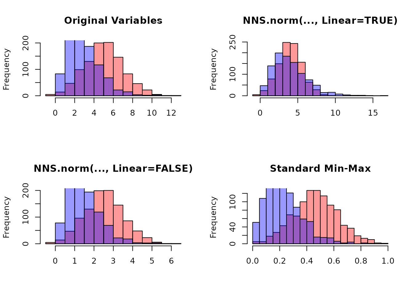
Quantile normalization forces distributions to be identical. This is literally the opposite intended effect of NNS.norm, which preserves individual distribution shapes while aligning ranges. The quantile normalized series become identical in distribution, while the NNS methods retain the original patterns.

Practical Applications

Normalization eliminates the need for multiple y‑axis charts and prevents their misuse. By placing variables on the same axes with shared ranges, we enable more relevant conditional probability analyses. This technique, combined with time normalization, is used in NNS.caus() to identify causal relationships between variables.

`NNS.rescale()`: Distribution Rescaling

NNS.rescale() performs one‑dimensional affine transformations.

Function signature:

NNS.rescale(x, a, b, method = "minmax", T = NULL, type = "Terminal")

1) Min-Max Scaling

If method = "minmax":

$x^{*} = a + (b - a) \frac{x - \min(x)} {\max(x) - \min(x)}$

Properties:

Preserves order
Maps support to $[a,b]$
Linear transformation

Example

raw_vals <- c(-2.5, 0.2, 1.1, 3.7, 5.0)

scaled_minmax <- NNS.rescale(
  x = raw_vals,
  a = 5,
  b = 10,
  method = "minmax",
  T = NULL,
  type = "Terminal"
)

cbind(raw_vals, scaled_minmax)
#>      raw_vals scaled_minmax
#> [1,]     -2.5      5.000000
#> [2,]      0.2      6.800000
#> [3,]      1.1      7.400000
#> [4,]      3.7      9.133333
#> [5,]      5.0     10.000000
range(scaled_minmax)
#> [1]  5 10

2) Risk-Neutral Scaling

If method = "riskneutral":

Let:

$S_0 = a$
$r = b$
$T$ = time horizon

Terminal Type

Target:

$\mathbb{E}[S_T] = S_0 e^{rT}$

Transformation form:

$x^{*} = x \cdot \frac{S_0 e^{rT}} {\text{mean}(x)}$

This enforces the required expectation.

Discounted Type

Target:

$\mathbb{E}[e^{-rT} S_T] = S_0$

Equivalent to:

$\mathbb{E}[S_T] = S_0 e^{rT}$

but the returned series is scaled so that its discounted mean equals $S_0$ . In practice, the function applies the same multiplicative factor as above, because:

$\text{mean}(e^{-rT} x^{*}) = e^{-rT} \cdot \text{mean}(x^{*}) = e^{-rT} \cdot S_0 e^{rT} = S_0.$

Risk-Neutral Example

set.seed(123)
S0 <- 100
r <- 0.05
T <- 1

# Simulate a price path
prices <- S0 * exp(cumsum(rnorm(250, 0.0005, 0.02)))

rn_terminal <- NNS.rescale(
  x = prices,
  a = S0,
  b = r,
  method = "riskneutral",
  T = T,
  type = "Terminal"
)

c(
  mean_original = mean(prices),
  mean_rescaled = mean(rn_terminal),
  target = S0 * exp(r * T)
)

mean_original mean_rescaled        target 
     109.7019      105.1271      105.1271

Discounted Example

rn_discounted <- NNS.rescale(
  x = prices,
  a = S0,
  b = r,
  method = "riskneutral",
  T = T,
  type = "Discounted"
)

c(
  mean_rescaled = mean(rn_discounted),
  target_discounted_mean = S0
)

         mean_rescaled target_discounted_mean 
                   100                    100

Conceptual Summary

`NNS.norm()`

Multivariate
Dependence‑aware scaling
Equalizes means only in linear mode
Preserves shape and order

`NNS.rescale()`

Univariate
Affine transformation
Either range‑targeted or expectation‑targeted
Preserves rank structure

Both functions maintain monotonicity and are therefore compatible with NNS copula and dependence modeling frameworks.

set.seed(123)

x <- rnorm(1000, 5, 2)
y <- rgamma(1000, 3, 1)

# Combine variables
X <- cbind(x, y)

# NNS normalization
X_norm_lin <- NNS.norm(X, linear = TRUE)
X_norm_nonlin <- NNS.norm(X, linear = FALSE)

# Standard min-max normalization
minmax <- function(v) (v - min(v)) / (max(v) - min(v))
X_minmax <- apply(X, 2, minmax)

References

If the user is so motivated, detailed arguments further examples are provided within the following:

Fred Viole