Getting Started with NNS: Correlation and Dependence

library(NNS)
library(data.table)
require(knitr)
require(rgl)

Correlation and Dependence

The limitations of linear correlation are well known. Often one uses correlation, when dependence is the intended measure for defining the relationship between variables. NNS dependence NNS.dep is a signal:noise measure robust to nonlinear signals.

Below are some examples comparing NNS correlation NNS.cor and NNS.dep with the standard Pearson’s correlation coefficient cor.

Linear Equivalence

Note the fact that all observations occupy the co-partial moment quadrants.

x = seq(0, 3, .01) ; y = 2 * x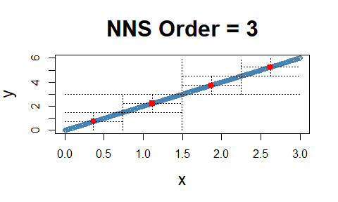

cor(x, y)

## [1] 1

NNS.dep(x, y)

## $Correlation
## [1] 1
## 
## $Dependence
## [1] 1

Nonlinear Relationship

Note the fact that all observations occupy the co-partial moment quadrants.

x = seq(0, 3, .01) ; y = x ^ 10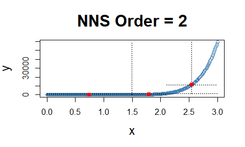

cor(x, y)

## [1] 0.6610183

NNS.dep(x, y)

## $Correlation
## [1] 0.9595032
## 
## $Dependence
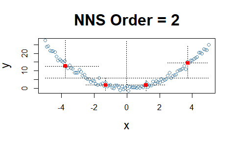
## [1] 0.9595032

Cyclic Relationship

Even the difficult inflection points, which span both the co- and divergent partial moment quadrants, are properly compensated for in NNS.dep.

x = seq(0, 12*pi, pi/100) ; y = sin(x)

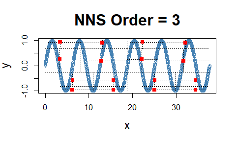
cor(x, y)

## [1] -0.1297766

NNS.dep(x, y)

## $Correlation
## [1] 0.2022363
## 
## $Dependence
## [1] 0.8207786

Asymmetrical Analysis

The asymmetrical analysis is critical for further determining a causal path between variables which should be identifiable, i.e., it is asymmetrical in causes and effects.

The previous cyclic example visually highlights the asymmetry of dependence between the variables, which can be confirmed using NNS.dep(..., asym = TRUE).

cor(x, y)

## [1] -0.1297766

NNS.dep(x, y, asym = TRUE)

## $Correlation
## [1] 0.2022363
## 
## $Dependence
## [1] 0.8207786

cor(y, x)

## [1] -0.1297766

NNS.dep(y, x, asym = TRUE)

## $Correlation
## [1] 0.07270847
## 
## $Dependence
## [1] 0.4086234

Dependence

Note the fact that all observations occupy only co- or divergent partial moment quadrants for a given subquadrant.

set.seed(123)
df = data.frame(x = runif(10000, -1, 1), y = runif(10000, -1, 1))
df = subset(df, (x ^ 2 + y ^ 2 <= 1 & x ^ 2 + y ^ 2 >= 0.95))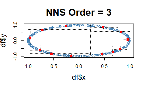

NNS.dep(df$x, df$y)

## $Correlation
## [1] 0.05834412
## 
## $Dependence
## [1] 0.46764

p-values for `NNS.dep()`

p-values and confidence intervals can be obtained from sampling random permutations of $y \rightarrow y_p$ and running NNS.dep(x,$y_p$) to compare against a null hypothesis of 0 correlation, or independence between $(x, y)$ .

Simply set NNS.dep(..., p.value = TRUE, print.map = TRUE) to run 100 permutations and plot the results.

## p-values for [NNS.dep]
set.seed(123)
x = seq(-5, 5, .1); y = x^2 + rnorm(length(x))

NNS.dep(x, y, p.value = TRUE, print.map = TRUE)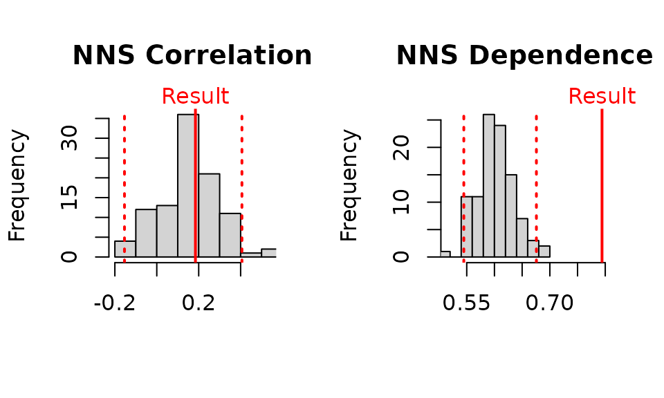

## $Correlation
## [1] 0.1844261
## 
## $`Correlation p.value`
## [1] 0.39
## 
## $`Correlation 95% CIs`
##       2.5%      97.5% 
## -0.1541078  0.4062421 
## 
## $Dependence
## [1] 0.794182
## 
## $`Dependence p.value`
## [1] 0
## 
## $`Dependence 95% CIs`
##      2.5%     97.5% 
## 0.5447205 0.6757430

Multivariate Dependence `NNS.copula()`

These partial moment insights permit us to extend the analysis to multivariate instances and deliver a dependence measure $(D)$ such that $D \in [0,1]$ . This level of analysis is simply impossible with Pearson or other rank based correlation methods, which are restricted to bivariate cases.

set.seed(123)
x = rnorm(1000); y = rnorm(1000); z = rnorm(1000)
NNS.copula(cbind(x, y, z), plot = TRUE, independence.overlay = TRUE)

## [1] 0.3278775

References

If the user is so motivated, detailed arguments and proofs are provided within the following:

Fred Viole