Getting Started with NNS: Normalization and Rescaling
Fred Viole
Source:vignettes/NNSvignette_04_Normalization_and_Rescaling.Rmd
NNSvignette_04_Normalization_and_Rescaling.RmdOverview
This vignette covers two related tools:
-
NNS.norm()for cross‑variable normalization when comparing multiple series. -
NNS.rescale()for single‑vector rescaling with either min‑max or risk‑neutral targets.
Both functions are deterministic rescalings.
NNS.rescale() is affine on a single vector and preserves
its rank structure. NNS.norm() multiplies each column by
its own factor, so it preserves the order within each column, but in
nonlinear mode a factor can be negative, which reverses that column’s
order and the sign of its correlations with the others (see the note
below).
NNS.norm(): Normalize Multiple Variables
NNS.norm() rescales variables to a common magnitude
while preserving distributional structure. The method can be
linear (all variables forced to have the same mean) or
nonlinear (using dependence weights to produce a more
nuanced scaling). In the nonlinear case, the degree of association
between variables influences the final normalized values.
Mathematical Structure
Let be an matrix of variables.
Step 3: Dependence Weight Matrix
If linear = FALSE:
- If number of variables :
- Otherwise:
NNS.dep()returns a symmetric matrix of nonlinear dependence measures.
If linear = TRUE, the weighting effectively becomes:
Nonlinear Case Interpretation
Thus, the normalized mean becomes a dependence‑weighted average of original means. Variables more strongly dependent with higher‑mean variables scale upward more.
Examples
Basic Multivariate Example
This holds for any distribution type and can be applied to vectors of different lengths. Each column is multiplied by a factor built from ratios of column means, so the columns should have positive means. A mean near zero, or of the opposite sign to the others, gives a very large or negative factor (see the note at the end of this vignette); the columns below are all positive.
set.seed(123)

A <- rnorm(100, mean = 5, sd = 1)
B <- rnorm(100, mean = 20, sd = 5)
C <- rnorm(100, mean = 10, sd = 1)
D <- rnorm(100, mean = 50, sd = 10)

X <- data.frame(A, B, C, D)

# Linear scaling
lin_norm <- NNS.norm(X, linear = TRUE, chart.type = NULL)
head(lin_norm)
     A Normalized B Normalized C Normalized D Normalized
[1,]     18.38264     17.81323     25.40626     18.19440
[2,]     19.75029     23.05113     23.56018     18.03539
[3,]     27.15749     20.32425     20.27462     17.24622
[4,]     20.99534     19.77814     21.95814     16.76224
[5,]     21.23872     16.50706     19.96390     19.37523
[6,]     27.80492     21.41627     19.83496     22.63783

# Verify means are equal
apply(lin_norm, 2, function(x) c(mean = mean(x), sd = sd(x)))

     A Normalized B Normalized C Normalized D Normalized
mean    21.077727    21.077727    21.077727    21.077727
sd       3.779676     5.236256     1.978297     4.410985
Each column keeps its coefficient of variation and its correlations with the others, because it is multiplied by a single positive factor.
Now compare with nonlinear scaling:
nonlin_norm <- NNS.norm(X, linear = FALSE, chart.type = NULL)
head(nonlin_norm)
     A Normalized B Normalized C Normalized D Normalized
[1,]     2.082162     4.690344     4.098285     11.04240
[2,]     2.237074     6.069519     3.800493     10.94589
[3,]     3.076072     5.351514     3.270500     10.46693
[4,]     2.378098     5.207720     3.542068     10.17321
[5,]     2.405665     4.346421     3.220377     11.75906
[6,]     3.149404     5.639050     3.199579     13.73917

apply(nonlin_norm, 2, function(x) c(mean = mean(x), sd = sd(x)))

     A Normalized B Normalized C Normalized D Normalized
mean    2.3874296     5.549909    3.4000486     12.79232
sd      0.4281159     1.378742    0.3191192      2.67708
Note that the means differ and the standard deviations are smaller than in the linear case, reflecting the dependence structure.
Normalize list of unequal vector lengths
set.seed(123)
vec1 <- rnorm(n = 10, mean = 0, sd = 1)
vec2 <- rnorm(n = 5, mean = 5, sd = 5)
vec3 <- rnorm(n = 8, mean = 10, sd = 10)

vec_list <- list(vec1, vec2, vec3)

NNS.norm(vec_list)

$`x_1 Normalized`
 [1]  13.074058  -3.004912 -11.745878  25.406891  -4.647966  -5.481229   6.225165   5.920719   6.113733   9.640242

$`x_2 Normalized`
[1]  2.875960212  0.008876158  1.230826150  5.855582361 10.779166523

$`x_3 Normalized`
[1]  4.0749062  2.2395840  0.4067264  0.7457562 15.6445780  5.1941416  2.3326665  2.5622994
Quantile Normalization Comparison
Quantile normalization forces distributions to be identical. This is
literally the opposite intended effect of NNS.norm, which
preserves individual distribution shapes while aligning ranges. The
quantile normalized series become identical in distribution, while the
NNS methods retain the original patterns.
Practical Applications
Normalization eliminates the need for multiple y‑axis charts and
prevents their misuse. By placing variables on the same axes with shared
ranges, we enable more relevant conditional probability analyses.
NNS.caus() places variables on a shared scale with
per-column ranks instead, so its results do not depend on the location
or units of either variable.
NNS.rescale(): Distribution Rescaling
NNS.rescale() performs one‑dimensional affine
transformations.
Function signature:
NNS.rescale(x, a, b, method = "minmax", T = NULL, type = "Terminal")1) Min-Max Scaling
If method = "minmax":
Properties:
- Preserves order
- Maps support to
- Linear transformation
Example
raw_vals <- c(-2.5, 0.2, 1.1, 3.7, 5.0)

scaled_minmax <- NNS.rescale(
  x = raw_vals,
  a = 5,
  b = 10,
  method = "minmax",
  T = NULL,
  type = "Terminal"
)

cbind(raw_vals, scaled_minmax)
#>      raw_vals scaled_minmax
#> [1,]     -2.5      5.000000
#> [2,]      0.2      6.800000
#> [3,]      1.1      7.400000
#> [4,]      3.7      9.133333
#> [5,]      5.0     10.000000
range(scaled_minmax)
#> [1] 5 10Risk-Neutral Example
set.seed(123)
S0 <- 100
r <- 0.05
T <- 1

# Simulate a price path
prices <- S0 * exp(cumsum(rnorm(250, 0.0005, 0.02)))

rn_terminal <- NNS.rescale(
  x = prices,
  a = S0,
  b = r,
  method = "riskneutral",
  T = T,
  type = "Terminal"
)

c(
  mean_original = mean(prices),
  mean_rescaled = mean(rn_terminal),
  target = S0 * exp(r * T)
)

mean_original mean_rescaled        target
109.7019 105.1271 105.1271 Conceptual Summary
NNS.norm()
- Multivariate
- Dependence‑aware scaling
- Equalizes means only in linear mode
- One factor per column: shape is preserved, and order too unless the factor is negative
NNS.rescale()
- Univariate
- Affine transformation
- Either range‑targeted or expectation‑targeted
- Preserves rank structure
NNS.rescale() is monotone increasing, so ranks, copulas
and NNS dependence measures are unchanged by it. NNS.norm()
is too when every factor is positive, but in either mode a column whose
mean has the opposite sign from the others gets a negative factor. For
example, with x ~ N(1, 1) and
y = x - 1.5 + noise, cor(x, y) is 0.957 before
NNS.norm() and -0.957 after; with x <- 1:4
and y <- x - 4, linear = TRUE turns a
correlation of 1 into -1 as well. Check the signs of the factors before
using normalized columns for dependence or causation.
set.seed(123)

x <- rnorm(1000, 5, 2)
y <- rgamma(1000, 3, 1)

# Combine variables
X <- cbind(x, y)

# NNS normalization
X_norm_lin <- NNS.norm(X, linear = TRUE)
X_norm_nonlin <- NNS.norm(X, linear = FALSE)

# Standard min-max normalization
minmax <- function(v) (v - min(v)) / (max(v) - min(v))
X_minmax <- apply(X, 2, minmax)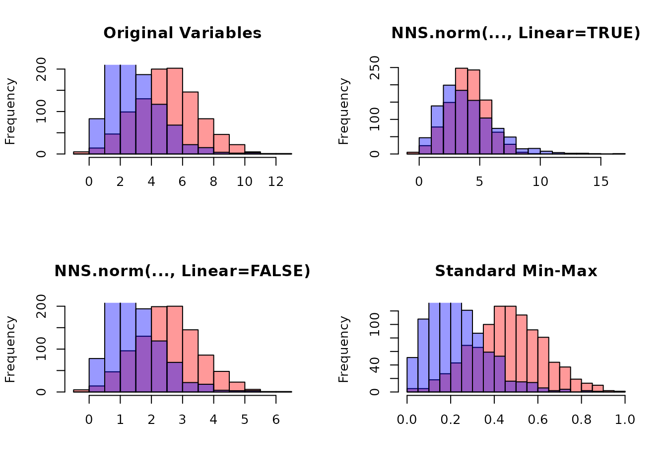
References
If the user is so motivated, detailed arguments further examples are provided within the following:
Nonlinear Scaling Normalization with NNS (archived PDF; see the current corrections and editable companion for the normalization qualifications).
Distributional Equivalence in GBM: Outcome Transformation for Efficient Risk-Neutral Pricing